4. Integration

This chapter is about the concept of integration. After completing the chapter you should be able to:

• Find the anti-derivative for standard problems by inspection

• Know the fundamental theorem of calculus

• Calculate the area under a curve by definite integration

4.1. The “anti-derivative”

Anti-differentation refers to the inverse of differentiation. For a given function the anti-derivative tells us the parent function that would have generated it through the process of differentiation. For example, since the cosine function can be obtained by differentiating the sine function, we can think of the sine function as cosine’s anti-derivative.

However, we cannot say that the anti-derivative is unique since for any constant \(c\) the following result holds:

(4.1)\[\begin{equation} \frac{\mathrm{d}}{\mathrm{d}x}\biggr(\sin(x)+c\biggr)=\cos(x) \end{equation}\]

Therefore, we write the following result, where \(\int{f(x)\mathrm{d}x}\) means taking the anti-derivative of \(f(x)\) and \(c\) is an arbitrary constant:

(4.2)\[\begin{equation} \int{\cos(x)}\mathrm{d}x = \sin(x)+c \end{equation}\]

Definition

In general, for a given function \(f(x)\),

\(\quad\) if \(\displaystyle \biggr[ \frac{\mathrm{d}F}{\mathrm{d}x} = f(x)\biggr]\), then \(\displaystyle\biggr[F(x)+c\biggr]\) is an antiderivative of \(x\),

where \(c\) is an arbitrary constant.

Being able to “spot” anti-derivatives is a tremendously useful (and often under-utilised) trick.

Exercise 4.1

Find anti-derivatives of the following functions:

\[\begin{align*} &\text{(a) } x^3 && \text{(b) } \sin(3x) && \text{(c) } e^{a x}\\ &\text{(d) } x \sqrt{x^2-1} \qquad \qquad && \text{(e) } \frac{x}{x^2+1} \qquad \qquad && \text{(f) }\frac{\sin(x)}{\cos(x)} \end{align*}\]

Note: these are not “integration questions”, you only need to use your knowledge of differentiation, and the concept of the anti-derivative, as described above.

Solution (a)

If we differentiate \(x^4\) we obtain \(4x^3\) which is nearly what we want, but not quite. Trying \(\displaystyle \frac{\mathrm{d}}{\mathrm{d}x} \left(\frac{1}{4} x^4\right)\) instead gets the result \(x^3\), and so the anti-derivative of \(x^3\) is

\[\begin{equation*} \int{x^3}\mathrm{d}x = \frac{1}{4} x^4+c \end{equation*}\]

Solution (b)

By the chain rule, \(\displaystyle \frac{\mathrm{d}}{\mathrm{d}x} \cos(3x)=-3\sin(3x)\), and so the anti-derivative is

\[\begin{equation*} \int{\sin(3x)}\mathrm{d}x = -\frac{1}{3}\cos(3x)+c \end{equation*}\]

Solution (c)

Since \(\displaystyle \frac{\mathrm{d}}{\mathrm{d}x}e^{a x}=a e^{a x}\) the anti-derivative is

\[\begin{equation*} \int{e^{ax}}\mathrm{d}x =\frac{1}{a} e^{a x}+c \end{equation*}\]

Solution (d)

Now we rely on our expertise with the chain rule, which tells us that

\[\begin{equation*} \int \frac{\mathrm{d}F}{\mathrm{d}u}\frac{\mathrm{d}u}{\mathrm{d}x}\mathrm{d}x = F(u)+c \end{equation*}\]

If we differentiate \(F(u)=u^{3/2}\) where \(u=x^2-1\), we obtain

\[\begin{equation*} \frac{\mathrm{d}F}{\mathrm{d}x}=\biggr[2 x\biggr]\biggr[\frac{3}{2} u^{1/2}\biggr] \end{equation*}\]

So, the anti-derivative that we require is

\[\begin{equation*} \int{x u^{1/2}\mathrm{d}x}=\frac{1}{3} u^{3/2}+c =\frac{1}{3} (x^2-1)^{3/2}+c \end{equation*}\]

Solution (e)

By the same rationale as the previous question, we try

\[\begin{equation*} \frac{\mathrm{d}}{\mathrm{d}x} \ln(x^2+1)=\frac{2x}{x^2+1} \end{equation*}\]

So, the anti-derivative is

\[\begin{equation*} \int{\frac{x}{x^2+1}\mathrm{d}x}=\frac{1}{2} \ln(x^2+1)+c \end{equation*}\]

Solution (f)

The anti-derivative is

\[\begin{equation*} \int{\frac{\sin(x)}{\cos(x)}\mathrm{d}x}=-\ln(\cos(x))+c \end{equation*}\]

In general, the anti-derivative of an expression of the form \(\displaystyle \frac{f^{\prime}(x)}{f(x)}\) is

\[\begin{equation*} \int{\frac{f^{\prime}(x)}{f(x)}\mathrm{d}x}=\ln(f(x))+c \end{equation*}\]

4.2. Area under the curve

Below, Fig. 4.1 shows how the area under a curve \(f(x)\) between \(x=a,b\) may be estimated by drawing rectangles of equal width.

Once Loop Reflect

Fig. 4.1 Rectangles drawn under the curve \(f(x)\) can be used to approximate the area. The thinner the rectangles, the better the approximation. Integration is equivalent to this approach as the width of the rectangles, \(\Delta x \rightarrow 0\).

The relationship between the number of rectangles and the width \(\Delta x\) is given by

(4.3)\[\begin{equation} \Delta x = \frac{b-a}{n} \end{equation}\]

The area of the rectangle with left-hand edge at \(x=x_n\) is given by \(f(x_n)\Delta x\), and it may be proved that by summing these in the limit we obtain

(4.4)\[\begin{equation} \text{Area} = \int_a^b f(x)\mathrm{d}x=F(b)-F(a) \end{equation}\]

where \(F(x)\) is the anti-derivative of \(f(x)\). We call this result the integral.

Fundamental theorem of calculus (FTC)

The link between area under the curve and the anti-derivative is known as the first FTC. The second FTC essentially proves that every continuous function has an anti-derivative, which can be found by integration.

For some functions, such as \(e^{-x^2}\) we might not be able to express the integral in terms of elementary functions, but we know it exists and we can use successive approximation techniques to estimate them either analytically or numerically.

Notation

\(\mathrm{d}x\) means “with respect to \(x\)

The integration is along the \(x\)-axis. We say that \(x\) is the integration variable. Do not forget to write this, or the integral has no meaning. The notation comes from the notional width of each rectangle being summed.

\(\int\) is the integration operator

An operator acts on a function in some way. For example, \(\frac{\textrm{d}}{\textrm{d}x}\) is also an operator.

\(f(x)\) is the integrand

The integrand is the function to be integrated.

\(a, b\) are the limits of integration

If the integral has limits then it is called a definite integral and has a single value for the solution. If the integration does not have limits then it is called an indefinite integral, and you can only compute the result to within an arbitrary constant.

Signed and unsigned areas

Note that the heights of the rectangles in Fig. 4.1 are given by \(f(x)\), and so if \(f(x)<0\) then the result will be negative. In many examples, positive and negative areas cancel. For instance,

(4.5)\[\displaystyle \int_0^{2\pi}\sin(x)\mathrm{d}x = 0 \textrm{, since } \displaystyle \int_0^{\pi}\sin(x)\mathrm{d}x = 2 \textrm{ and } \displaystyle \int_{\pi}^{2\pi}\sin(x)\mathrm{d}x = -2\]

If you want the total (unsigned) area between the curve and the axis, then you can work with the modulus of the function,

(4.6)\[\displaystyle \int_a^b |f(x)|\mathrm{d}x\]

The easiest way to do this is to split up the region of integration into areas where \(f(x)>0\) and areas where \(f(x)<0\). For example,

(4.7)\[\displaystyle \int_0^{2\pi}|\sin(x)|\mathrm{d}x = \displaystyle \int_0^{\pi}\sin(x)\mathrm{d}x+ \displaystyle \int_{\pi}^{2\pi}-\sin(x)\mathrm{d}x = 2+2 =4\]

The results are illustrated in Fig. 4.2:

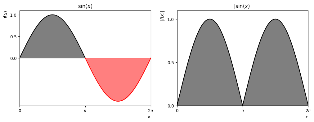
Fig. 4.2 [Left] The black and red signed areas (2,-2) cancel when the integral is performed; [Right] The black signed are both positive and so the integral is 2+2=4.

Similarly, if we perform the integration along the x-axis in the negative direction, then the quantities \(\Delta x\) are negative, and so we end up with a negative signed area when \(f(x) > 0\).

FTC1 also confirms that \(\displaystyle \int_b^a f(x) \textrm{d}x = -\displaystyle \int_a^b f(x) \textrm{d}x\).

Area between two curves

Where \(f(x) \geq g(x)\) the integral \(\displaystyle \int (f(x)-g(x)) \textrm{d}x\) gives the area between the two curves. An example is shown below:

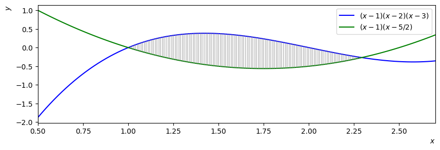
Fig. 4.3 Can you find the enclosed area?

Solution

The two curves intersect when \(x=1\), \(x=3-1/\sqrt{2}\). Therefore the enclosed area is given by

\[\begin{equation*} \int_1^{3-1/\sqrt{2}}x^3-6x^2+\frac{17}{2}\mathrm{d}x = \frac{13}{48}+\frac{\sqrt{2}}{3} \end{equation*}\]

4.3. Integral of \(\displaystyle \frac{1}{x}\)

By inspection, we can deduce the following general result for the polynomial anti-derivative:

(4.8)\[\begin{equation} \int x^n \mathrm{d}x = \frac{x^{n+1}}{n+1} +c, \qquad (n\neq -1) \end{equation}\]

The result for the special case \(n=-1\) can be deduced from the properties of the natural logarithm:

(4.9)\[\begin{equation} \frac{\mathrm{d}}{\mathrm{d}x}\Big(\ln(x)\Big) = \frac{1}{x} \quad \implies \quad \int \frac{1}{x}\mathrm{d}x=\ln(x)+C \end{equation}\]

However, this result is only valid for the case when \(x>0\) since the natural logarithm is not defined for \(x<0\). On the other hand, the integral for negative values of \(x\) can be inferred from the symmetry of the reciprocal function, as shown in the plot below:

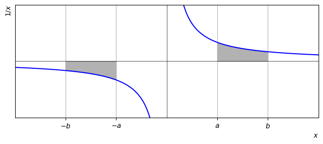
We see that:

\[\int_{-b}^{-a}\frac{1}{x}\mathrm{d}x = -\int_a^b\frac{1}{x}\mathrm{d}x = \int_b^a\frac{1}{x}\mathrm{d}x = \int_{-b}^{-a}\frac{1}{|x|\mathrm{d}x}\]

Hence, we can write down the following more general result, which holds for all \(x\), provided that the range of integration does not cross the vertical axis:

(4.10)\[\begin{equation} \int\frac{1}{x}=\ln(|x|)+\mathrm{const} \end{equation}\]

Formally \(\displaystyle \int_{-a}^a\frac{1}{x}\mathrm{d}x\) is undefined, although we can define what is called the Cauchy principal value of this integral as:

\[\lim_{\epsilon\rightarrow 0^{+}}\left( \int_{-a}^{-\epsilon}\frac{1}{x}\mathrm{d}x+ \int_{\epsilon}^a\frac{1}{x}\mathrm{d}x\right)=0\]

4.4. Mean value of a function

The average of a discrete function is given by adding up the values and dividing by the number of points. We extend this concept to continuous functions in the limit as \(\Delta x\rightarrow 0\), as illustrated in the plot below:

Once Loop Reflect

Fig. 4.4 We can obtain the average output \(\bar{f(x)}\) by adding up the datapoints and dividing by the number of datapoints used.

By taking the limit as \(\Delta x\rightarrow 0\), we can obtain the average of a continuous function \(f(x)\) and we find that this result is equal to the limit defintion of the definite integral.

(4.11)\[\begin{equation} \bar{f} = \frac{1}{b-a} \int_a^b f(x)\mathrm{d}x \end{equation}\]

For example, to calculate the mean value of \(\cos ^3(\theta)\) on the interval \(\displaystyle \left[-\frac{\pi}{3}, \frac{\pi}{3}\right]\) by integration:

(4.12)\[\begin{align} \frac{1}{\frac{\pi}{3} - \left(-\frac{\pi}{3}\right)} \int_{-\pi/3}^{\pi/3}\cos^{3}(\theta)\mathrm{d}\theta &= \frac{3}{2\pi}\displaystyle \int_{-\pi/3}^{\pi/3}\cos(\theta)(1-\sin^2(\theta))\mathrm{d}\theta\\ &=\frac{3}{2\pi}\left[\sin(\theta)-\frac{1}{3}\sin^3(\theta)\right]_{-\pi/3}^{\pi/3} = \frac{9\sqrt{3}}{8\pi} \end{align}\]

Exercise 4.2

1. Find the average value of the function \(f(x) = x^3\) on the interval \(x \in [0,\, 1]\).

2. Find the mean value of the cosine function on the interval \(x \in \Big[0,\, \frac{\pi}{2}\Big]\).

Solution

1.

\[\begin{equation*} \bar{f} = \frac{1}{1-0} \int_0^{1} x^3\,\mathrm{d}x = \int_0^{1} x^3\,\mathrm{d}x = \Big[ \frac{x^4}{4}\Big]_0^{1} = \frac{1}{4} \end{equation*}\]

2.

\[\begin{equation*} \bar{f} = \frac{1}{\frac{\pi}{2}-0} \int_0^{\pi/2} \cos(x)\,\mathrm{d}x = \frac{2}{\pi} \int_0^{\pi/2} \cos(x)\,\mathrm{d}x = \frac{2}{\pi}\,\Big[ \sin(x)\Big]_0^{\pi/2} = \frac{2}{\pi} \end{equation*}\]