3. Derivative applications

This chapter is about applying differentiation to find tangents and stationary points. The latter problem is especially important, as minimisation problems are of great interest to scientists.

After completing the chapter you should be able to:

• find the equation of the tangent at a given point on a curve

• find and classify stationary points of functions

3.1. Tangent and normal

Recall that the equation of the line passing through a given point \((x_0,y_0)\) with slope \(m\) is given by:

\[\begin{equation*} \frac{y-y_0}{x-x_0}=m \qquad \text{i.e} \qquad y=m(x-x_0)+y_0. \end{equation*}\]

This result is essentially a mathematical statement of the fact that the slope of a line is constant.

Tangent

The tangent line at a given point \((x_0,y_0)\) on a curve is defined as the line with the same slope as the curve. The equation is therefore given by the following result, in which the notation \([]_{x=x_0}\) means that the enclosed expression is evaluated at \(x=x_0\).

(3.1)\[\begin{equation} \frac{y-y_0}{x-x_0}=m, \qquad m=\left[\frac{\mathrm{d}y}{\mathrm{d}x}\right]_{x=x_0} \end{equation}\]

Below we use this definition to plot the tangent to the curve \(y=x^2\).

Show calculation

The analytic derivative of \(y=x^2\) is given by

\[\begin{equation*} \frac{\mathrm{d}y}{\mathrm{d}x}=2x \end{equation*}\]

Therefore the tangent equations are given by:

• At the point \((0.2,0.04)\)

\[\begin{equation*} \frac{y-0.04}{x-0.2}=0.4 \quad \implies \quad y=0.4x-0.04 \end{equation*}\]

• At the point \((1.2,1.44)\)

\[\begin{equation*} \frac{y-1.44}{x-1.2}=2.8 \quad \implies \quad y=2.8x-1.92 \end{equation*}\]

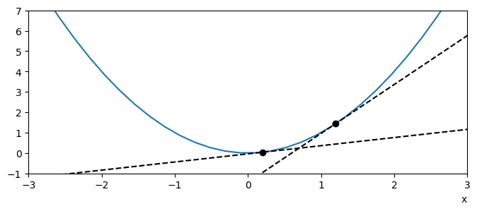
Fig. 3.1 \(y=x^2\) and its tangent at \(x=0.2,\ 1.2\)

Normal

The gradient of the normal (perpendicular) line to the tangent is \(-1/m\). The equation of the normal line is therefore given by

(3.2)\[\begin{equation} \quad \frac{y-y_0}{x-x_0}=-\frac{1}{m} \qquad m=\left[\frac{\mathrm{d}y}{\mathrm{d}x}\right]_{x=x_0} \end{equation}\]

Justification of the result

The relationship between the slopes of the tangent and normal can be observed from the similarity of the two illustrated triangles below:

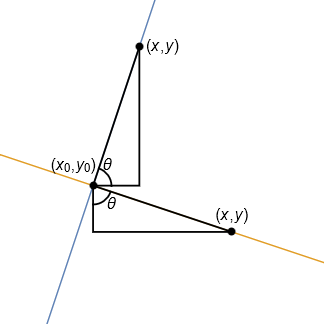
Let \(\theta\) be the illustrated angle and define \(m=\tan(\theta)\), representing the gradient of the blue line.

The equation of the perpendicular line is therefore given by

\[\begin{equation*} m= \frac{x-x_0}{-(y-y_0)} \implies \frac{y-y_0}{x-x_0}=-\frac{1}{m} \end{equation*}\]

Exercise 3.1

Differentiate \(y=x^4-2x^2\) and hence

(i) Calculate the equation of the tangent to this curve at \(x=3\)
(ii) Calculate the equation of the normal to the curve at \(x=3\)

Solution

We are interested in the point \((3,63)\) and at this point

\(\displaystyle \left[\frac{\mathrm{d}y}{\mathrm{d}x}\right]_{x=3}=\biggr[4x^3-4x\biggr]_{x=3}=4(3^3)-4(3)=96\)

(i) The tangent to the curve at the point satisfies

\(\displaystyle \frac{y-63}{x-3}=96 \quad \implies \quad y=96x-225 \)

(ii) The normal to the curve at the point satisfies

\(\displaystyle \frac{y-63}{x-3}=\frac{-1}{96} \quad \implies \quad y=\frac{-1}{96}x+\frac{2017}{32} \)

It is also possible to get these results from Wolfram Alpha. For example, you can type:

• “line tangent to y=x^2 at x=0.2”

• “line normal to y=x^4-2x^2 at x=3”

Warning

Sometimes it might take a little bit of experimenting to see if you can get the results that you want from Wolfram Alpha. For example, the following may give something unexpected!

• “tangent of y=x^4-2x^2 at x=3”

3.2. Stationary points

In some applications we need to find points where the rate of change of a function \(y(x)\) is zero. At these so-called “stationary points” the curve representing the function is flat. By way of example, we will consider the function plotted below.

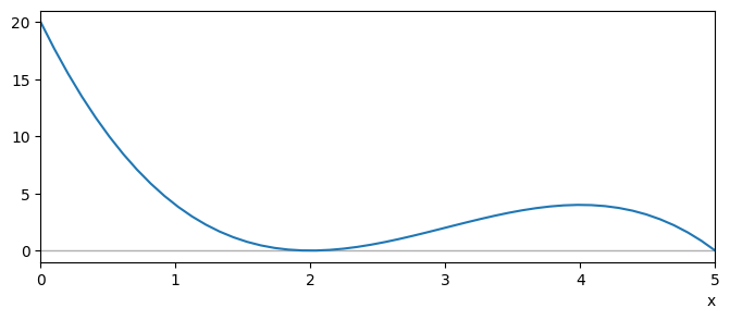
Fig. 3.2 \(y(x)=-x^3+9x^2-24x+20\) on the domain \([0,5]\)

It is clear from the plot that there is a local minimum and a local maximum. We can verify the location of these points by differentiation:

\[\begin{align*} y^{\prime}(x)&=-3 x^2+18x-24 \\ &= -3(x-2)(x-4), \qquad y^{\prime}(x)=0 \implies x=2,4. \end{align*}\]

It is also possible to solve some problems of this sort with Wolfram Alpha. For example:

• “stationary points of -x^3+9x^2-24x+20”

• “roots of -3x^2+18x-24”

Classification by hand

We can classify stationary points without the use of a plot by looking algebraically at the slope of the curve either side of each stationary point. This can be useful if we want to find general results that do not rely on producing a plot for each scenario.

It is convenient to record the results in a table, as demonstrated below for the function plotted in Fig. 3.2. We know that the gradient changes sign only at the points \(x=2,4\), so we can conveniently choose the test points as follows.

Table 3.1 Sign change for \(y=-x^3+9x^2-24x+20\)

	\(x=1\)	\(x=2\)	\(x=3\)	\(x=4\)	\(x=5\)
\(y^{\prime}(x)\)	-	0	+	0	-

From the table, we can infer that \(x=2\) is a local minimum and \(x=4\) is a local maximum.

Exercise 3.2

Can you guess the sign of the second derivative at the points \(x=2,4\) ?

Solution

The second derivative measures the rate of change of the slope \(s\), since

\[\begin{equation*} \frac{\mathrm{d}^2y}{\mathrm{d}x^2} =\frac{\mathrm{d}}{\mathrm{d}x}\frac{\mathrm{d}y}{\mathrm{d}x}=\frac{\mathrm{d}s}{\mathrm{d}x}, \end{equation*}\]

• When \(y^{\prime\prime}(x)>0\) the slope is increasing

• When \(y^{\prime\prime}(x)<0\) the slope is decreasing

Since the slope at \(x=2\) is going from negative to positive, the second derivative at this point will be positive (increasing).

Since the slope at \(x=4\) is going from positive to negative, the second derivative at this point will be negative (decreasing).

We can therefore use the second derivative to classify local maxima/minima. However, this test is not conclusive for the case when the second derivative is equal to zero.

In addition to maxima and minima we have the possibility of another type of stationary point called a point of inflection. This occurs when the slope of a function becomes zero without changing sign. The most basic example of an inflection point is for the function \(y=x^3\), which is stationary at \(x=0\). Plots of the function and its derivative are illustrated below:

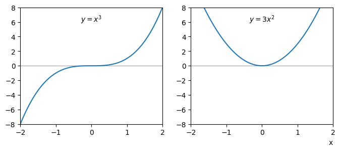
Fig. 3.3 [Left] The cubic has an inflection point at \(x=0.\)

The table below shows how the sign either side of the stationary point.

Table 3.2 Sign change for \(y=x^3\)

	\(x=-1\)	\(x=0\)	\(x=1\)
\(y^{\prime}(x)\)	+	0	+

Exercise 3.3

Show that the following function has a stationary point at \(x=2.\) What does the result \(y^{\prime\prime}(2)\) tell you about this point? Is this point a local maximum/minimum/inflection?

\[\begin{equation*} y(x)=x^4-8x^3+24x^2-32x+23 \end{equation*}\]

Solution

\(y^{\prime}(x)=4x^3-24x^2+48x-32\)
\(\implies y^{\prime}(2)=32-96+96-32=0\)

\(y^{\prime\prime}(x)=12x^2-48x+48\)
\(\implies y^{\prime\prime}(2)=48-96+48=0\)

This result doesn’t tell us anything about the stationary point! It could be a local maximum/minimum or a point of inflection.

In this case the slope is increasing either side of the stationary point, so the point is a minimum:

\(y^{\prime\prime}(x)=12(x^2-4x+4)=12(x-2)^2 \geq 0 \ \forall x\)

Wolfram Alpha also has the answer

3.3. Gompertz

The Gompertz function can be used in various modelling scenarios, such to model population growth, spread of disease and growth of tumours. It is given by

\[\begin{equation*} y = a e^{-be^{-ct}}, \qquad a,b,c>0. \end{equation*}\]

A plot of the curve is shown below for particular values of \(a,b,c\).

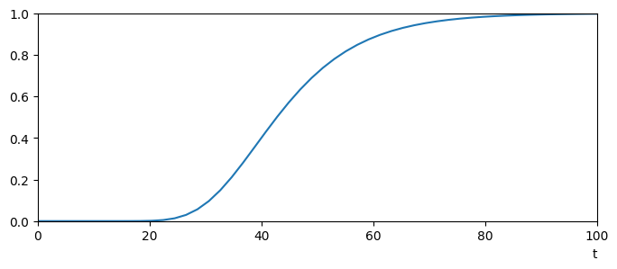
Show that \(y^{\prime\prime}=0\) when \(t=\ln(b)/c\). What is the significance of this result?