
2. Rates of change#
Much of what we do in the natural sciences is concerned with studying the relationships between variables. We often consider the effect of changing one variable upon the other, which we call the dependent variable. For instance, we might consider how changing CO2 levels affect global temperatures, how student debt grows over time, or the way that a drug binds to biological receptors as a function of the chemical concentration. This chapter is about how we report and analyse changes in these relationships over time.
After completing the chapter you should be able to:
Use a linear rate-of-change estimate to estimate missing data such as a future value, and also recognise the dangers involved in doing so.
Calculate rate of change estimates on an interval-by-interval basis for a dataset or function
Find the instantaneous rate of change of a given function, by using the idea of allowing the interval to shrink to zero.
2.1. Linear estimate#
The rate of change of a measurement \(y(x)\) over an interval is obtained by dividing the absolute growth by the width of the interval:
Geometrically, this represents the slope of the line connecting two points at the start and end of the interval of interest. If the relationship \(y(x)\) is nonlinear as shown in the plot below, then the statistic is an averaged value
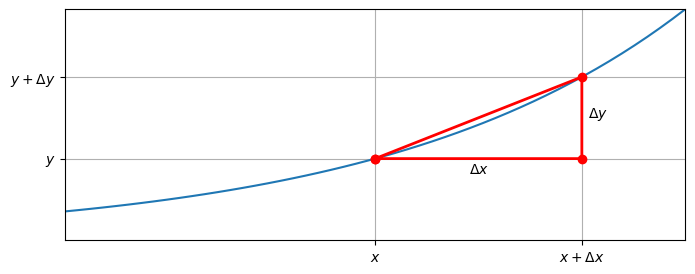
Fig. 2.1 The rate of change of \(y(x)\) over the interval shown is given by the slope of the line connecting the end-points of the interval.#
If the rate of change stays relatively constant over consecutive intervals, then we can use this fact to make inferences about the future value of the dependent variable. We do this quite naturally in our day-to-day activities - such as guesstimating how long a bathtub will take to fill at a given rate, how long a cup of tea will take to cool, or how long it will take to reach our journey destination at the current speed.
Exercise 2.1
Suppose that you are studying a new blood pressure drug. At a dose of 5mg the slope of the dose-response curve is -2 mmHg/mg. Approximately how much would a patient’s blood pressure change if the drug dose was increased to 5.1mg?
Solution
According to the information given in the question, blood pressure decreases by 2mmHg per mg increase in dose. Thus, for a 0.1mg increase in dose we expect blood pressure to decrease by 0.2mmHg.
We can write out the calculation mathematically as follows:
Let \(R\) be the response and \(D\) be the dose, and let \(\Delta R,\ \Delta D\) represent changes in these quantities. According to the information given in the question,
Taking \(\Delta D=0.1\text{mg}\) then gives
The blood pressure would decrease by 0.2mmHg.
Treating the slope as constant is usually a reasonable approximation when looking at small changes. However, if the rate of change varies significantly then we may need to take this variation into account.
If we have access to data over shorter intervals, then we can compare estimates of the rate of change for each period, to test for consistency, as demonstrated in the following example.
Tik Tok
From its launch in September 2016, TikTok gained 1.037 billion new monthly active users (MAUs) worldwide by September 2021 [Business of apps]
Denoting the number of active MAUs by \(n\) and the time by \(t\), we can write down an expression for the growth rate over the period, which we can also convert to a monthly statistic:
However, this result is an averaged value. We can use company data shown in the table below to calculate the monthly growth rates using shorter measurement periods, and compare these to the average.
Sep’16 |
Mar’18 |
Jun’18 |
Sep’18 |
Dec’18 |
Mar’19 |
Jun’19 |
Sep’19 |
|
|---|---|---|---|---|---|---|---|---|
\(t\) (month) |
0 |
18 |
21 |
24 |
27 |
30 |
33 |
36 |
\(n\) (million) |
0 |
85 |
133 |
198 |
271 |
333 |
381 |
439 |
Dec’19 |
Mar’20 |
Jun’20 |
Sep’20 |
Dec’20 |
Mar’21 |
Jun’21 |
Sep’21 |
|
\(t\) (month) |
39 |
42 |
45 |
48 |
51 |
54 |
57 |
60 |
\(n\) (million) |
508 |
583 |
700 |
667 |
756 |
812 |
902 |
1037 |
Try calculating the growth rates for each period and when you are ready to reveal the answers
The calculations show that there is some variation in the monthly growth rates over the period. Plotting the data can also give us an attractive overview. From the plot we can see that growth over the first 18 months to March 2018 was relatively slow, followed by a period to September 2021 that is characterised fairly well by a linear growth rate of 22.67 million MAUs / month, despite variations in the data.
The model function is given by the following equation, where the number of monthly active users \(n\) is measured in millions:
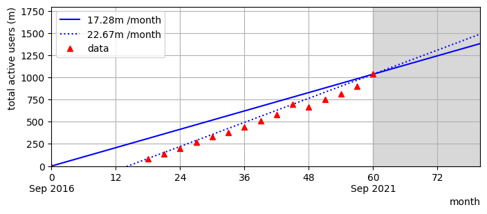
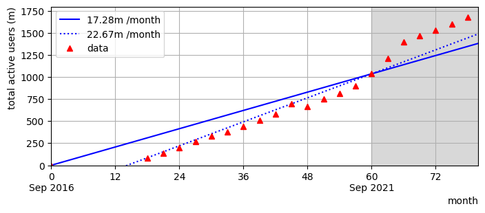

Fig. 2.2 Tik Tok MAUs in millions (m). To show/hide data for December 2021 to March 2023 #
When we observe growth that looks linear like this it is tempting to assume that the trend will continue in future. However, we should be cautious unless we have good reason to believe in the validity of the linear model. In this case the linear model predicts that from September 2021 to March 2023 Tik Tok would gain an additional 0.408 billion active user. The actual data reported a gain of 0.64 billion users, exceeding the model’s prediction by over 50%.
2.2. Interpolation#
In the above example the growth rate was relatively constant and so we were able to use a linear model of the following form, where \(m\) represents the growth rate/slope:
However, many relationships are not linear. We will now move on to construct a more general growth rate model. We will suppose that the measurement can be modelled by some function \(y(x)\) which, may be nonlinear. The model could come frome theoretical considerations, or from empirical observations. For example, let us consider a model in which the relationship between two variables is given by
The growth rate (slope) of this function is not constant. However, if we pick any two points on the curve we can find the average growth rate over the corresponding interval. For instance, between \(x=1\) and \(x=2\), the average growth rate is given by the slope of the line connecting these two points:
By choosing the intervals to be not too large we can obtain a good representation of how the growth rate changes with \(x\).
The graph below illustrates the principle, in which we approximate the curve \(y(x)\) by joining up a set of representative points with straight lines. This is known as a “linear interpolation”. By increasing the number of points over the domain we obtain a result that appears smoother and more like the model function.
Fig. 2.3 Approximating the function \(y=x^2\) using a linear interpolation with \(n\) datapoints.#
It is helpful to label the points using a subscript notation:
The slope of each line segment is then given by
For example, if we represent the curve \(y=x^2\) using five data points in the interval \(0\leq x \leq 4\) then we obtain four line segments. The slopes of these line segments are presented in the data table below. We can see how the slope increases with \(x\).
Notice that the estimate of the slope at \(x=4\) has not been computed. You could do this if you wanted to, though it would require using the endpoint from the next interval \((5,25)\).
\(x\) |
\(y\) |
\(\Delta x\) |
\(\Delta y\) |
\(m\) |
|---|---|---|---|---|
0 |
0 |
1 |
1 |
1 |
1 |
1 |
1 |
3 |
3 |
2 |
4 |
1 |
5 |
5 |
3 |
9 |
1 |
7 |
7 |
4 |
16 |
- |
- |
- |
We can do this for any smooth function, and by taking smaller differences \(\Delta x\) we obtain a better representation of how the slope changes.
Exercise 2.2
Complete by hand for the case where \(y=x^3\)
\(x\) |
\(y\) |
\(\Delta x\) |
\(\Delta y\) |
\(m\) |
|---|---|---|---|---|
0.0 |
||||
0.5 |
||||
1.0 |
||||
1.5 |
||||
2.0 |
Solution
\(x\) |
\(y\) |
\(\Delta x\) |
\(\Delta y\) |
\(m\) |
|---|---|---|---|---|
0.0 |
0.000 |
0.5 |
0.125 |
0.25 |
0.5 |
0.125 |
0.5 |
0.875 |
1.75 |
1.0 |
1.000 |
0.5 |
2.375 |
4.75 |
1.5 |
3.375 |
0.5 |
4.625 |
9.25 |
2.0 |
8.000 |
- |
- |
- |
We cannot complete the final row unless we use the next point, which is (2.5,15.625)
2.3. Instantaneous rate#
For a changing function the averaged growth rate (2.7) depends on the interval \(\Delta x\), but we are interested in the growth rate as the interval size shrinks to zero. If we think of \(x\) as a time-like variable, this tells us how much the function is changing on a moment-by-moment basis as illustrated in the plot below.
Fig. 2.4 As we reduce the interval width \(\Delta x\) the slope approaches its “instantaneous” value.#
Numerically we cannot take \(\Delta x=0\) since “0/0” is indeterminate. However, we can try some small values. For instance, for the squared function, we can estimate the growth rate at the point \(y=1\) using some intervals of successively smaller width:
\(\Delta x\) |
\(y(1+\Delta x)\) |
\(\Delta y\) |
\(m=\Delta y/\Delta x\) |
|---|---|---|---|
1 |
4 |
3 |
3 |
0.1 |
1.21 |
0.21 |
2.1 |
0.01 |
1.0201 |
0.0201 |
2.01 |
0.001 |
1.002001 |
0.002001 |
2.001 |
0.0001 |
1.00020001 |
0.00020001 |
2.0001 |
These results seem to be converging (approaching) to a value of 2. We can understand why this is the case by using algebra to work out slope for an arbitrary value of \(\Delta x\) :
Substituting \(x=1\) into this expression and choosing the appropriate values of \(\Delta x\) gives us the values in the right-hand column of our table.
However, what is really exciting here is that the result gives us the instantaneous slope of the squared function for any value of \(x\). By allowing the interval \(\Delta x\) to shrink to zero we obtain
The arrow notation here means that the expression on the left tends to (approaches) the expression on the right. We call this result the derivative of \(x^2\).
Exercise 2.3
Use the approach outlined in this section to show that the derivative of the function \(y=x^3\) is given by \(3x^2\).
Solution
As \(\Delta x\) shrinks to zero, the result tends to \(3x^2\).