3. Exponential trends

Exponential growth is constant factor growth. It appears in many real-life contexts such as compound interest where the amount of interest is a percentage of the cash amount; and population growth where the number of births per capita remains fairly constant over the short term.

In the real world exponential growth is normally time-limited. For example, it may be constrained by resource availability or regulation. However, understanding exponential growth is an essential first step towards building more realistic models.

After working through this chapter you should be able to:

• Produce by hand a rough plot of the exponential function for any base \(k\).

• Calculate the relative growth rate of a dataset or function and link this to exponential growth.

• Recognise the key growth rate property of the natural exponent \(e\)

3.1. Doubling

Suppose that you are convinced by a get-rich-quick scheme that promises to double your money every year. If you invest £5 in the scheme, how much money do you expect to have after 4 years? How much would you have after \(n\) years?

Solution

According to the claims of the scheme you should expect to have:

\[\begin{equation*} y=£5\times 2\times 2 \times 2\times 2 = £5\times 2^4 = £80. \end{equation*}\]

After \(n\) years you would have \(y=£5\times 2^n\).

The double-your-money scheme involves repeated multiplication by a constant factor. The result has the general form given below, in which \(y_0\) is the initial value, \(k\) is the multiplication factor and \(n\) is the number of years.

(3.1)\[\begin{equation} y_n=y_0 k^n \end{equation}\]

The multiplication factor is also known as the base and the model can be called exponential in base \(k\). In the get-rich-quick example the initial investment was \(y_0=£5\) and base was \(k=2\).

Where have we seen this before?

We have seen relationships of this type in the chapter on growth models, where \(r\%\) annual growth was modelled by taking \(\displaystyle k=\biggr(1+\frac{r}{100}\biggr)\).

How does it look?

A plot of the exponential relationship \(y=2^x\) is shown below. It can be seen from the plot that the curve is shallow for small values of \(x\), and steep for larger \(x\). For comparison, a plot of \(y=x^2\) is also shown. You can adjust the slider in the plot to see more of the curves by extending the axes.

Once Loop Reflect

Fig. 3.1 A comparison of polynomial growth (degree 2) with exponential growth (factor 2).

By \(x=5\) the exponential \(2^x\) has already outpaced the quadratic \(x^2\). The exponential function continues to grow tremendously and by \(x=30\) the doubling function has already reached more than one billion, whilst the squared function has only reached 900.

We therefore see that doubling growth can be quite dramatic. In fact, it can be shown that the doubling function will eventually outpace a polynomial of any degree.

A famous example of doubling growth is Moore’s Law. It is not really a law, but actually an observation, or guiding principle, related to the manufacture of computer chips. The ‘law’ has held true for the last 50 years, which has been a crucial factor in the computing explosion that has enabled us to carry pocket devices today with more computing power than the supercomputers of the 1980s.

3.2. Change of base

We can relate growth in any base to the doubling function by rescaling the \(x\) axis. For example, consider the exponential with base \(k=1.01\), which corresponds to a growth rate of one percent:

(3.2)\[\begin{equation} y=1.01^x \end{equation}\]

This function grows very slowly in comparison to the doubling function. By \(x=70\) it has only just doubled. We may use this fact to note that a growth rate of 1% is equivalent to stretching out the doubling function by a factor of 70 in the \(x\)-direction:

(3.3)\[\begin{equation} y=(1.01^{70})^{x/70} \simeq 2^{x/70} \end{equation}\]

The same analysis can be applied to any base \(k\geq 1\), where the stretching factor \(s\) is the solution to the problem \(k^s=2\). We will learn how to solve this problem in another chapter, but for now we can get an approximate solution by trial and error.

For instance for base \(k=1.2\), we may note that

(3.4)\[\begin{equation} k^3 < 2 < k^4 \end{equation}\]

Therefore the function \(1.2^x\) can be obtained from the doubling function by a stretch in the \(x\)-direction that has a scale factor somewhere between 3 and 4.

The plot below shows how the exponential in different bases can be related to the doubling function by rescaling the \(x\)-axis.

Once Loop Reflect

Fig. 3.2 Adjust the slider to plot \(y=k^x\) for different values of \(k\). The change of base corresponds to a rescaling of the \(x\)-axis, so the curve stays the same whilst the values on the horizontal axis change.

We could relate the exponential in any base to any other base. In these examples, we have chosen to focus on base 2 because the doubling function is perhaps the easiest exponential to conceptualise.

Exercise 3.1

What is the relationship between growth in base 3 and growth in base 10?

Solution

Since \(3^2<10<3^{2.1}\), growth in base 3 is the same as growth in base 10 stretched in the \(x\)-direction by a factor slightly bigger than 2.

Exponential decay
In the example above the multiplication factor \(k\) was greater than one. If the multiplication factor is in the range \(0<k<1\) then the value of the function depreciates (decreases). We call this exponential decay.

For example, when \(k=0.5\) we have a “halving function” instead of a doubling function. The graph of the halving function can be obtained by reflecting the doubling function in the \(y\)-axis as shown in the figure below. This may be understood from the laws of exponents:

(3.5)\[\begin{equation} 0.5^x = \left(\frac{1}{2.0}\right)^x = 2.0^{-x} \end{equation}\]

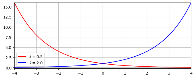
Fig. 3.3 Exponential function \(y=k^x\) for different values of \(k\).

Exercise 3.2

Which function should be reflected in the \(y\)-axis to obtain the graph of \(0.80^x\) ?

Solution

We should reflect the graph \(y=1.25^x\). This may be seen by writing:

\[\begin{equation*} 0.80^x = \left(\frac{1}{0.80}\right)^{-x}=1.25^{-x} \end{equation*}\]

3.3. Growth rate

We can produce a table of values to calculate the absolute and relative growth rates between points of our choosing. In the table below this is done for the exponential \(y=2^x\) using five points that are each separated by an amount \(\Delta x=0.5\).

Table 3.1 Averaged growth rates for \(y=2^x\)

\(x\)	\(y\)	\(\Delta x\)	\(\Delta y\)	\(\displaystyle \frac{\Delta y}{\Delta x}\)	\(\displaystyle \frac{1}{y}\frac{\Delta y}{\Delta x}\)
1.0	2.00	0.5	0.83	1.66	0.83
1.5	2.83	0.5	1.17	2.34	0.83
2.0	4.00	0.5	1.66	3.32	0.83
2.5	5.66	0.5	2.34	4.68	0.83
3.0	8.00	-	-	-	0.83

It is immediately striking that the relative growth rate is constant. This should not be very surprising, since exponential growth represents an increase or decrease by the same proportion over each same-size measurement interval.

Mathematically, the relative growth rate of the exponential in base \(k\) is given by:

(3.6)\[\begin{equation} \frac{1}{y}\frac{\Delta y}{\Delta x} = \frac{k^{\Delta x}-1}{\Delta x} \end{equation}\]

Proof

\[\begin{equation*} \frac{\Delta y}{\Delta x} = \frac{y(x+\Delta x)-y(x)}{\Delta x} = \frac{k^{x+\Delta x}-k^x}{\Delta x} = \frac{k^x(k^{\Delta x}-1)}{\Delta x} \end{equation*}\]

We can simplify the expression on the right if we convert this to a relative growth rate:

\[\begin{equation*} \frac{1}{y}\frac{\Delta y}{\Delta x} = \frac{1}{k^x} \frac{k^x(k^{\Delta x}-1)}{\Delta x} = \frac{k^{\Delta x}-1}{\Delta x} \end{equation*}\]

This result depends only on the base \(k\) and the chosen interval \(\Delta x\). Crucially it is the same at all \(x\) locations.

In this example, taking \(k=2\) and \(\Delta x =0.5\) gives us a result that is about \(0.83\), consistent with our calculations. Taking smaller intervals gives a result closer to the “instantaneous” relative growth value of the doubling function:

(3.7)\[\frac{2^{0.000001}-1}{0.000001}\simeq 0.693\]

The natural exponent

Different values of \(k\) will give different relative growth rates, which begs the following question:

Exercise 3.3

For what value of \(k\) is the instantaneous relative growth rate equal to one? See if you can find an approximate answer using trial and error.

Solution

The result to 3 decimal places is 2.718. This is our first approximation to the “natural exponent” \(e\).

\[\begin{equation*} \frac{2.718^{0.000001}-1}{0.000001}\simeq 0.9999 \end{equation*}\]

This value is called the “natural” exponent \(e\). It satisfies the following result as the interval \(\Delta x\) approaches zero.

(3.8)\[\begin{equation} \frac{e^{\Delta x}-1}{\Delta x} \quad \to \quad 1 \end{equation}\]

The natural exponent can also be used to model exponential relationships with relative growth rates that are not equal to one. Consider an expression of the following form, where \(\lambda\) is a constant:

\[y=e^{\lambda x}\]

The relative growth rate is given by the result below, where the final expression is obtained by making a substitution \(q=\lambda \Delta x\).

\[\begin{equation*} \frac{1}{y}\frac{\Delta y}{\Delta x}=\frac{e^{\lambda \Delta x}-1}{\Delta x}=\lambda \frac{e^q-1}{q} \end{equation*}\]

We want to evaluate this expression as \(\Delta x\) approaches zero, which is the same as allowing \(q\) to approach zero. Therefore:

what’s in a name

The relative growth rate of \(e^{\lambda x}\) is \(\lambda\). This explains why \(e\) is considered the “natural” exponent to use in problems involving continuous compound growth.