4. Logarithms

We now turn our interest to the inverse of the exponential function, which poses the following problem:

Given a certain value \(y\), what value of \(x\) satisfies the relationship \(y=e^x\) ?

We will need to solve this problem to do algebra involving exponentials. Defining the exponential without its inverse would be like defining multiplication without division. In non-mathematical terms it would be like having the ability to put your shoes on but no way to take them off again!

After working through this chapter you should be able to:

• Manipulate logarithms and use them to “find the unknown” in problems involving exponentials

• Recognise why it might be useful to use a logplot, and give an example of where they might be used

4.1. Definition

Thinking about the (input,output) relationship of the exponential function, we can see that the inverse (output,input) graph can be obtained by swapping the \(x\) and \(y\) axes. This is equivalent to a reflection in the line \(y=x\), as shown in the figure below. This relationship with the inverse is true for all functions. For example, the graph of the square root function can be obtained by reflecting the squared function in the line \(y=x\).

We call the inverse of the (natural) exponential function the natural logarithm, and we denote it by \(\ln(x)\).

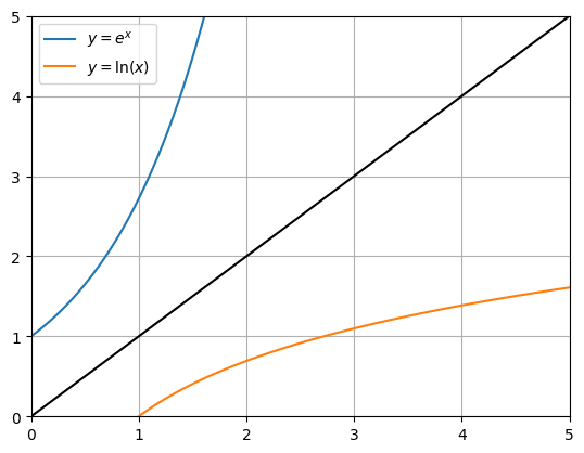
Fig. 4.1 The exponential function together with its inverse.

We can get an estimate of the natural logarithm by reading off from the graph. For instance, we can see that \(e^x=2\) is obtained when \(x\) is roughly equal to 0.7. We can obtain a more precise result by bracketing the value:

\(x\)	\(e^x-2\)
0.6931	-
0.6932	+

The value lies between (0.6931,0.6932) so we can conclude that it is 0.693 to 3 decimal places. Your calculator can give you a more accurate value for ln(2).

We can also find the logarithm in different bases, using the notation \(\ln_k\). For the logarithm in base 10, the subscript is often omitted. Due to the way that we have defined the logarithm as the inverse of the exponential function we can say that the following two expressions are logically equivalent, as indicated by the symbol \(\iff\), which can be read as “implies and implies that”:

(4.1)\[\begin{equation} y=\log_k(x) \quad \iff \quad k^y=x. \end{equation}\]

Exercise 4.1

Without using a calculator, what is the value of
(a) \(\log{100}\qquad\) (b) \(\log{1000}\qquad\) (c) \(\ln_3{27}\)

Solution

(a) The answer is 2, since \(10^2=100\)
(b) The answer is 3, since \(10^3=1000\)
(c) The answer is 3, since \(3^3=27\)

We use logarithm in base 10 when we want to think in decimal terms (e.g. finance) or about orders of magnitude. The logarithm in base \(e\) is used much more frequently in sciences, due to the self-equivalent growth rate property of the natural exponent.

4.2. Useful results

We can combine the exponential and logarithm into a single result, which highlights the way that inverse functions work:

(4.2)\[x=e^{\ln(x)} \qquad \text{ or } \qquad x=\ln(e^{x}).\]

In either of the two forms above, we see that applying one function followed by its inverse takes us back to where we started. In non-mathematical terms it’s like putting your shoes on and then taking them off again.

We can use this result to derive some further relationships.

Change of base

The following result shows that \(k^x\) is obtained by stretching out \(e^x\) by a factor of \(\ln(k)\)

(4.3)\[k^x=\left(e^{\ln(k)}\right)^x = e^{\lambda x}, \quad \lambda=\ln(k)\]

Exercise 4.2

Can you use this finding to explain the result given in (3.7), which showed that the relative growth rate of \(2^x\) is roughly 0.693 ?

Solution

According to our finding at the end of the chapter on exponentials, the relative growth rate of \(e^{\lambda x}\) is \(\lambda\)

We have now shown that \(2^x\) is equivalent to \(e^{\lambda x}\) where \(\lambda=\ln(2)\), therefore the relative growth rate of \(2^x\) is equal to \(\ln(2)\), which is 0.693, given to 3 decimal places.

We can also use (4.3) to obtain a result that relates the log in base \(k\) to the natural logarithm:

(4.4)\[\begin{equation} \log_k(x) = \frac{\ln(x)}{\ln(k)} \end{equation}\]

Proof

To derive the result we start by writing out the following equivalent relationships:

\[\begin{equation*} y=\log_k(x) \quad \iff \quad x=k^y=e^{\ln(k)y} \end{equation*}\]

Taking the logarithm of both sides in the final expression then gives the result:

\[\begin{equation*} \ln(x)=y\ln(x) \quad \iff \quad y=\frac{\ln(x)}{\ln(k)}. \end{equation*}\]

Laws of logarithms

We can use the relationship between the exponential function and its inverse to derive the following three results, which apply in any base. The proofs of these results are not given, but are similar to those given above.

• \(\log(ab) = \log(a)+\log(b)\)

• \(\log(x^n) = n\log(x)\)

• \(\log(a/b) = \log(a)-\log(b)\)

Problems for you to try

[1] Write the expression \(\log(32)-3\log(4)+\log(3)\) as a single logarithm

Solution

\(\log\left(\frac{32\times 3}{4^4}\right)=\log\left(\frac{3}{2}\right)\)

[2] Find the value of \(x\) for which \(\log_2(x^2+4x+3)-\log_2(x^2+x)=4\)

Solution

\(\log_2\left(\frac{x^2+4x+3}{x^2+x}\right)=4\) gives \(\frac{x^2+4x+3}{x^2+x}=2^4\).

This which rearranges to a quadratic with solutions \(x=-1\), \(x=1/5\).

The negative solution is not applicable. Why?

[3] Solve the problem \(3^x=8\) by taking logarithms

Solution

\(x\log(3)=\log(8)\) gives \(x=\frac{\log(8)}{\log(3)}=1.89\) (3sf)

[4] Calculate the result \(\log_7(29)\) in terms of the natural logarithm

Solution

\(\log_7(29)=\frac{\ln(20)}{\ln(7)}\) or we can solve this problem as follows:

Let \(y=\log_7(29)\). Then \(7^y=29\).

Using \(7=e^{\ln(7)}\) gives \(y\ln(7)=29\) from which the result is immediately obtained.

[5] Solve the problem \(\log(x)+\ln(x)=2\)

Solution

\(\frac{\ln(x)}{\ln(10)}+\ln(x)=2\) gives \(\ln(x)=\frac{2\ln(10)}{1+\ln(10)}\),

So \(x=\exp\left(\frac{2\ln(10)}{1+\ln(10)}\right)=4.03\) (3sf)

[6] The hyperbolic cosine function is defined as \(\cosh(x)=\frac{1}{2}(e^x+e^{-x})\). By rewriting the equation \(\cosh(x)=4\) as a disguised quadratic in \(e^x\), solve to find the two possible values of \(x\). Give your answers as exact values involving the natural logarithm.

Solution

The given problem is \(\frac{1}{2}(e^x+e^{-x})=4\).

By taking \(y=e^{x}\) we can write this as \(y+\frac{1}{y}=8\).

This can be rearranged as \(y^2-8y+1=0\) with solutions \(y=4\pm \sqrt{15}\).

Since \(y=e^{x}\) the solutions to the given problem are \(x=\ln(4\pm\sqrt{15})\).

4.3. Logplots

If a given variable spans several orders of magnitude then when we plot it on a linear scale we may find that the plot is not very easy to read. In that case it may be helpful to plot one of the variables on a logarithmic scale. We normally use a base 10 logarithmic scale as we are more familiar with scale visualisations using powers of 10.

Two examples are given below.

Earthquakes

The Gutenberg-Richter (GR) law predicts that in any given region and time period, the number of earthquakes that are at least Richter magnitude \(x\) is given by the following relationship, where \(\alpha,\beta\) are constants:

\[N_x=\alpha e^{-\beta x}\]

Therefore a plot of \(\ln(N_x)\) against \(x\) is expected to follow a decreasing linear trend. Taking the natural logarithm of the proposed relationship gives

\[\ln(N_x)=\ln(\alpha)-\beta x\]

The plot below is based on 8,402 Richter scale measurements for magnitude 3+ earthquakes that were recorded in California from 1960 to 2014. These data were downloaded from the U.S Geological Survey www.usgs.gov. A straight line has been fitted to the data, from which the constants \(\alpha\) and \(\beta\) can be estimated. The data appear to fit the GR law very well!

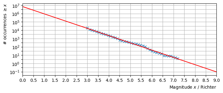
It can be seen from the graph that every unit increase in the Richter value corresponds to approximately a factor 10 decrease in the number of earthquakes.

Exercise 4.3

Estimate the value of \(\beta\) using the plot. Note that the vertical axis uses a scale that is logarithmic in base 10, whilst the GR is logarithmic in base \(e\).

Solution

We can use two points forming a triangle, such as the one illustrated below:

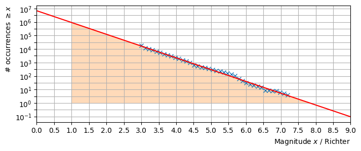
From the triangle,

\[\begin{equation*} \beta\sim \frac{\ln(10^6)-\ln(10)^0}{7.8-1}=2.03 \end{equation*}\]

The estimated value of \(\alpha\) can be read from the vertical axis, though this is a bit difficult to obtain accurately.

Molecular binding

A biological sample with a concentration of \(N\) receptors per mg of tissue is immersed in a solution containing a drug (ligand) at concentration \(c\).

We may partition the receptor concentration into bound and free receptors per mg of tissue, using subscripts to denote these concentrations:

(4.5)\[N=N_b+N_f\]

According to the ‘lock and key’ model, the ligand (key) binds to the receptors (locks) in proportion to the concentration of receptors that remain free and to the ligand concentration. We may write this as follows where \(k_a\) is the constant of proportionality for the reaction, which is called the affinity constant:

(4.6)\[N_b = k_a c N_f\]

By substituting for \(N_f\) from (4.5) and rearranging, we obtain

(4.7)\[N_b=\frac{k_a c N}{1+k_a c} =\frac{c N}{k_d+c}, \qquad k_d=1/k_a.\]

The value \(k_d\) introduced in the rearrangement is called the dissociation constant. Notice that \(k_d\) must have the same dimensional units as \(c\) in order for the units in the equation to balance. The concentration is typically measured in molarities (M=mol/l). For more information, see (e.g) this paper

A plot of \(N_b\) as a function of the concentration \(c\) is shown below, for particular values of the other constants.

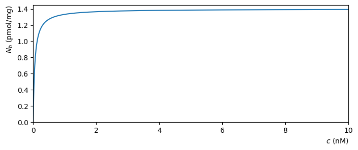
Fig. 4.2 Molecular binding as a function of concentration, for \(k_d=0.05\text{ nM}\) and \(N=1.4\text{ pmol/mg}\)

It can be seen that the receptors approach full occupancy \(N_b=N\) as the concentration increases. This can be anticipated from (4.7), by writing

\[\begin{equation*} N_b = \frac{cN}{k_d+c} = \frac{N}{1+k_d/c} \end{equation*}\]

As \(c\) becomes large, the ratio \(k_d/c\) shrinks towards zero and so \(N_b\) approaches \(N/(1_0)\). We will examine this idea in more detail when we study limits.

At half occupancy, \(N_b=N/2\), which gives

\[\begin{equation*} \frac{1}{2}=\frac{c}{k_d+c} \quad \Rightarrow k_d=c \end{equation*}\]

We see that the dissociation constant has the nice property that it is equal to the concentration at which half the receptors are bound.

It would be nice to illustrate this on the plot, but everything is bunched up near to the left-hand side. We can spread things out by plotting the horizontal axis values on a logarithmic scale, as shown below:

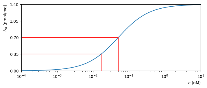
Fig. 4.3 Molecular binding as a function of logscale concentration. The red lines indicate the concentrations required for \(N_b=N/2\) and \(N_b=N/4\).

The horizontal axis has been scaled so that powers of 10 are equally spaced. This is useful for reading off data at lower concentrations. For this reason, logscale plots are sometimes used in molecular biology.

Warning

Although logscale plots are useful for illustrating data across a range of scales, they can be difficult to interpret as they change the shape of the plotted data. For example, the apparent inflection point shown in Fig. 4.3 is an artifical feature introduced by taking the log of the concentration values.