
1. Growth models#
Music on vinyl [BPI]
The purchase of albums on vinyl grew for a 15th consecutive year in 2022, [to] £119.5 million, up 3.1% on the year. The biggest-selling albums on the format were led by Taylor Swift’s Midnights, Harry Styles’ Harry’s House […] and The Car by Arctic Monkeys.
This chapter provides an introduction to concepts and depictions of growth. After working through the chapter you should
Understand the difference between absolute and relative growth and be able to calculate these two statistics for given data
Be able to distinguish between relative growth and percentage-point growth and decide when it is appropriate to use either measure
Calculate the average annual growth in absolute and relative terms, and write down models fitting these measurements.
Say whether you think an absolute or relative growth model is appropriate for a given dataset or scenario, with justification.
1.1. Measures of growth#
There are two princpal ways that we measure growth:
Absolute growth
This refers to the measured change in a quantity, in number of units. For example, if a plant leaf has increased in length from 3.6cm to 5.2cm then the absolute measure of growth is 1.6cm. A negative value would mean that the measurement quantity has decreased.
We can write down a formula for the absolute growth of a measurement \(y\) as follows, where \(y_0\) is the initial value and \(y_1\) is the final value. In the example case described above, these values are 3.6cm and 5.2cm, respectively:
Relative growth
This refers to a growth measurement that is given as a fraction or percentage, rather than a number of units. For example, an increase in length from 3.6cm to 5.2cm could be described in relative terms as a 44.4% increase.
We can convert our absolute growth formula to a relative growth formula by expressing it as a proportion of the initial measurement. This is called a growth factor :
Notice that the growth factor does not depend of the unit of measurement, due to unit cancellation between the numerator and denominator.
To obtain the result as a percentage value we simply multiply by 100. A growth factor of 1 is therefore equivalent to a 100% increase.
Test your understanding of relative growth by answering the following questions before you move on.
Exercise 1.1
If the growth factor is 2, which of the following statements are true about the measurement?
(there may be more than one answer):
| (a) it has doubled | (b) it has increased two-fold | (c) it has increased by its original size |
| (d) it has tripled | (e) it has increased three-fold | (f) it has increased twice its original size |
Solution
(b,d,f) are the true statements. If the relative growth factor is two, this means that the measurement has increased by twice its original size. This can also be described as a two-fold increase. Adding twice the size to the original size gives a result that is three times the original size!
Exercise 1.2
In 2005 the total public student loan debt of English domiciled students and EU students studying in England was £13.033 billion. By 2022 this figure had risen to £181.612 billion. Calculate both the absolute and relative growth during this period.
solution
Denoting the public student debt by \(y\) (in £billions), the absolute growth is
Converting this to a relative growth measure shows that this is a whopping 13-fold increase!
In percentage terms, the increase is about 1300%.
Exercise 1.3
In 2017 the estimated world population of southern white rhinos was 18,064. By 2021 it had fallen by about 11.7%. Approximately what was the population in 2021?
Solution
Using the formula for relative growth:
Taking \(y_0=18,064\) gives an esimate of around 15,950.
1.2. Percentage point growth#
Percentage point growth refers to the absolute difference between two percentages or proportions. For example, if the percentage of students who passed an exam increased from 85% to 90%, this would represent a five percentage point increase in the pass rate.
We report changes in this way when we are interested in the actual increase or decrease in a percentage, rather than the relative change or proportion compared to a base value.
To illustrate the difference between relative growth and percentage point growth, consider the following data which show the number of full-time undergraduate students enrolled at UCL vs any UK HE provider. The figures are derived from HESA data.
2014/15 |
2021/22 |
|
|---|---|---|
UCL |
15,350 |
23,020 |
All UK |
1,438,765 |
1,728,210 |
We can see that between 2014/15 and 2021/22 the number of students enrolled at UCL increased by 7,670 and that this represents a 50% uplift. Here, we used a percentage to report a relative increase in the number of UCL students.
However, in the same period of time, UCL’s share of the student population only increased from 1.067% to 1.332%, which is an increase of 0.265 percentage points. Here, we used a percentage to report an absolute increase in the proportion of students who are at UCL.
It is sometimes useful to report changes in a percentage or proportion in relative terms. However, you should take care, because “percentages of percentages” can be difficult to interpret or state correctly!
For example, the increase from 1.067% share to 1.332% share represents a 24.9% increase in UCL’s share of the undergraduate population. We can infer that some other universities must have larger proportional increases in student numbers over the time period of the data, since UCL’s student numbers went up by half whilst its share of the undergraduate population increased by only a quarter.
Exercise 1.4
The following statistics on UK voter intentions were provided by a YouGov survey
March 2020 |
March 2023 |
|
|---|---|---|
Conservative |
52% |
23% |
Labour |
28% |
45% |
Based on these statistics, calculate the increase in labour voting intentions over the period. State your answer both in percentage-point terms and in relative terms. Which of these measures do you think is most appropriate here?
Solution
percentage points:
45-28=17
Labour’s share of voting intentions increased by 17 percentage points.
Relative change:
17/28=0.607
Labour’s share of voting intentions increased by 60.7%
To avoid potential confusion for readers, it would be more accurate and clearer to state the absolute increase of 17 percentage points rather than using the percentage change. This approach provides a more straightforward representation of the change in Labour voting intentions over the given period.
1.3. Annual growth models#
We may be interested to compare growth amount over time. These comparisons can be done in absolute or relative terms as best fits the data and the purpose of the analysis.
If the data indicates consistent absolute growth every year then it would be appropriate to use an absolute measure. If the data indicates a consistent growth factor or proportional change then a relative measure would be more suitable.
The table below shows an example, based on annual data for full-time undergraduate students at UCL. In the second and third rows the growth between consecutive years is calculated using the data from the first row:
2014/15 |
2015/16 |
2016/17 |
2017/18 |
2018/19 |
2019/20 |
2020/21 |
2021/22 |
|
|---|---|---|---|---|---|---|---|---|
Number |
15,350 |
16,755 |
17,405 |
18,285 |
18,675 |
19,145 |
21,700 |
23,020 |
Growth |
1,405 |
650 |
880 |
390 |
470 |
2,555 |
1,320 |
- |
% |
9.153% |
3.879% |
5.056% |
2.132% |
2.517% |
13.346% |
6.083% |
- |
For this dataset the Average Annual Growth (AAG) is found to be:
\(k=1,096\) students in absolute terms
\(r=6.02\%\) in relative terms
We can compare the observed pattern of actual student numbers to a model based on either of these statistics.
Absolute growth model
In this model we will assume consistent absolute growth of \(k\) units per year. We use \(y_n\) to denote the measurement value in the \(n\)th year, with \(y_0\) representing the first measurement. We may then write down a general result, describing a linear relationship:
In our example where \(y\) represents student numbers at UCL, the initial value is \(y_0=15,350\) and \(k=1,096\) based on the AAG. We can produce a table and plot to compare the data with the model. If we think the model is a good fit to the data then we can potentially use it to predict future student numbers.
2015/16 |
2016/17 |
2017/18 |
2018/19 |
2019/20 |
2020/21 |
2021/22 |
|---|---|---|---|---|---|---|
16,446 |
17,542 |
18,638 |
19,734 |
20,830 |
21,926 |
23,022 |
Relative growth model
In this model we assume consistent percentage increase of \(r\%\) per year. We use \(y_n\) to denote the measurement value in the \(n\)th year, with \(y_0\) representing the first measurement. We may then write down a set of relationships between each measuement and the one before it:
By combining these results, we obtain a general formula for the measurement value in the \(n\)th year:
In our example where \(y\) represents student numbers at UCL, the initial value is \(y_0=15,350\) and \(r=6.02\%\) based on the AAG. We can produce a table and plot to compare the data with the model. If we think the model is a good fit to the data then we can potentially use it to predict future student numbers.
2015/16 |
2016/17 |
2017/18 |
2018/19 |
2019/20 |
2020/21 |
2021/22 |
|---|---|---|---|---|---|---|
16,274 |
17,253 |
18,292 |
19,393 |
20,561 |
21,799 |
23,111 |
Estimating validity
Plotting the model estimates together with the data can give us an indication of how good the model is. The figure below does this for our student numbers data. You can toggle between two different versions of the plot showing estimates based on either the absolute or relative growth model.
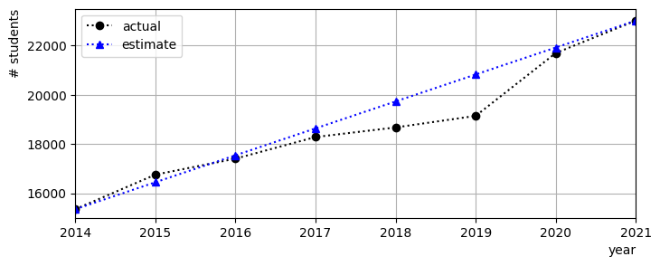
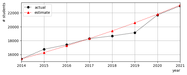

Fig. 1.1 Actual student numbers compared to estimates based on 1,096 additional students each year
To change the estimate #
From the plots there does not appear to be much to suggest that either model is significantly better in this case. This is not altogether surprising, since the function \((1+r/100)^n\) is close to linear over the short term if \(r\) is small. The decision on which model to use may therefore need to be based on theoretical reasoning, for instance about how UCL student recruitment works.
Exercise 1.5
If we do not have data available for all years, we can estimate an annual growth factor using only the first measurement \(y_0\) and last measurement \(y_n\) by rearranging (1.5). Use this approach to estimate \(r\) for the student number data. How does this compare to what we found using the AAG? Which measure do you think is better?
Solution
From (1.5) we obtain
This estimate is called the Compound Annual Growth (CAG) formula. For our student number data, we obtain
The result is pretty close to the AAG that we calculated, suggesting that our model of a constant growth factor should be a fairly good fit over the period of the data.
However, we should be very cautious when using the CAG formula to estimate an annual growth rate, since it relies on the model assumption that the growth factor is constant. If we have annual data available then we should find the annual growth rates so that we test this claim.
Warning
It is very important that we exercise caution when projecting a growth model into the future as there is significant possibility that future outcomes may deviate or differ from what the model predicts.
The fact that data fits a model is no guarantee that the model assumptions are correct or that the model includes any key factors that could influence the future growth, such as resource limitations.
Case study: student loan
This case study on student loans is provided for you to practice evaluating whether data fit a linear or exponential growth model.
The table below shows how the amount of student debt in England has changed since 2005. Data are obtained from House of Commons Student Loan Statistics [page 35, table 2].
\(t\) (year) |
2005 |
2006 |
2007 |
2008 |
2009 |
2010 |
2011 |
2012 |
2013 |
|---|---|---|---|---|---|---|---|---|---|
\(y\) (£ million) |
13033 |
15322 |
18116 |
21944 |
25963 |
30489 |
35186 |
40272 |
45903 |
\(t\) year |
2014 |
2015 |
2016 |
2017 |
2018 |
2019 |
2020 |
2021 |
2022 |
\(y\) (£ million) |
54355 |
64735 |
76253 |
89344 |
104457 |
121813 |
140093 |
160594 |
181612 |
Exercise 1.6
Public student debt in England has increased by around 1300% over a 17 year period. Which of the following do you think is closest to the annual (per year) growth rate over this period?
| (a) 76% | (b) 17% | (c) 2% | (d) 1% |
Solution
The answer is (b) 17%.
If you went for answer (a) this is probably because you divided the total percentage increase by the number of years. However, this is not how compound growth works.
Let us suppose that the student debt grows by 76% in the first year. In that case, the total balance at the beginning of the first year would be given by
The amount owed at the end of the second year would be given by 76% growth on the first year value
Continuing in this manner we find that the amount owed at the end of the \(n\)th year would be given by
Taking \(n=17\) gives a result of £ 194,428,420 B. This is about 500 times greater than the combined global wealth!
On the other hand, with a 17% growth rate we obtain
This figure is only about 0.05% of combined global wealth. It is also pretty close to the figure of £181.162B that is given in the table.
These calculations assume that growth is proportional, which is a pretty significant assumption.
Exercise 1.7
Use the figures given in the table to find the annual growth rates
in absolute terms (£)
in relative terms (%)
Solution
aaa
\(t\) (year) |
2005 |
2006 |
2007 |
2008 |
2009 |
2010 |
2011 |
2012 |
2013 |
|---|---|---|---|---|---|---|---|---|---|
\(y\) (£ million) |
13033 |
15322 |
18116 |
21944 |
25963 |
30489 |
35186 |
40272 |
45903 |
\(t\) year |
2014 |
2015 |
2016 |
2017 |
2018 |
2019 |
2020 |
2021 |
2022 |
\(y\) (£ million) |
54355 |
64735 |
76253 |
89344 |
104457 |
121813 |
140093 |
160594 |
181612 |
For this dataset the absolute growth rates are certainly not constant! However, the relative growth rates turn out to be quite similar. Try calculating the relative growth rates yourself and when you are ready to reveal the answers
Exercise 1.8
Based on the absolute and relative growth values that you found above, decide whether student loan debt can be best described by a linear or exponential model.
Use a graphing programme such as Desmos to produce a plot of student loan debt against time, based on your model.
Solution
The above results suggest growth by a consistent percentage amount every year. Taking the average of the values gives a growth rate of around 16.78%.
A plot of the data compared to the constant relative growth model is shown below. The model function is given by the following equation, where the debt \(D\) is measured in £billions. Notice that in this example the exponent is \((t-t_0)\) to account for the fact that the measurements started in 2005.
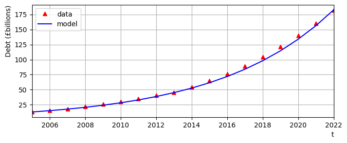
Fig. 1.2 Public student loan debt data, compared to an annual growth rate of 16.8%.
#
Exercise 1.9
If the historic growth trend continues, in what year will student loan debt reach twice the figure that it is today?
Solution
If the growth rate remains roughly constant (as it has done over the last 17 years) we can expect that the student loan debt will reach twich its current value in five years, since \(1.168^5\) gives a result that is a bit bigger than 2.
Note: If you inspect the table values you will also see that students loan debt has doubled roughly every five years.