QTHEN: 4. A representation for heat exchanger network configurations
A previous post discussed the use of cutting and splitting operations for the two-dimensional representation of hot and cold streams as the basis for the design of heat exchanger networks. In this post, I describe how to incorporate these operations in a bi-level optimization approach.
Bi-level optimization
Given a set of n streams defining the heat exchanger network synthesis problem, cutting and splitting create a set of n+1 streams, replacing one stream with a pair of streams. Each set of streams defines a design problem which we can evaluate using the graphical layout algorithm. We therefore consider a bi-level optimization problem. The outer problem determines the set of cutting and splitting operations. Each point in the search space (see below for representation of design points) of this outer level requires the solution of an inner optimization problem.
![\[ \min_{c \in \mathcal{C}, l \in \mathcal{L}} F(c,l) \]](ltximg/20251003_93c2f183df3af37d92361d2d3c2769c79db129d5.png)
subject to
![\[ l \gets \underset{\lambda \in \mathcal{L}(c)}{\arg \min} f(\lambda) \]](ltximg/20251003_74da82867d00679d8cf8dd68701b0dde29d049a8.png)
where c represents configurations which include different cuts and splits and l are layouts, defined as the order to place the streams in the two dimensional representation. The objective functions F and f are typically, for this problem, the same function.
Representation
The key is to define the possible search space for the outer optimization problem. We need to define a representation of alternative configurations, a representation which covers the search domain of interest effectively and efficiently. Effective means that all, or at least most, of the solutions of interest can be represented. Efficient means that solutions that are not of interest will not be represented or will form a small percentage of the search domain defined.
There are a couple of properties of the HEN problem that can be used to identify potential suitable representations. The first is that it is unlikely that there will be many cuts or splits so I am happy to start with no such operations and possibly add an operation to an existing configuration to create a new configuration. The second is that I do not believe there is much interest in cuts or splits that generate very small streams, noting that every stream will have at least one heat exchanger associated with it. The cost of a heat exchanger typically has a significant fixed cost contribution that is not dependent on the actual size. Small streams will lead to expensive outcomes generally.
Finally, it would be good to re-use existing representations, especially those that have already been shown to be effective for use with Fresa, my solver of choice.
The final representation I propose is a fixed size set of operations. The representation has to determine
- whether to cut, to split, or, in fact, do nothing;
- the amount of the duty to cut or split; and,
- which stream to cut or split.
Each operation will consist of a binary or boolean variable, with 0 (or false) indicating a cut operation and 1 (or true) a split operation. The operation will also have a quantity, η, which is the fraction of the stream to define either the cut or the split. The first segment in the cut will have a duty of η × Q, where Q is the total duty of that stream. The first branch of a split will have a flow given by the same value, η × Q.
To avoid small streams, I could constrain η to be ∈ [α, 1-α] for some small α ≪ 1, say. However, I also want to have any operation be excluded, acting as a NO-OP (no operation). The approach I will consider is that when η ∈ [0,1] \ [α,1-α], the operation is a NO-OP. This means not requiring more information in the definition of an operation beyond the binary/boolean variable and the cut or split fraction to represent the cases I am interested in.
Lastly, the operation has to operate on a stream. This could be represented by an index into the vector of streams. However, the set of streams will change in size depending on the operations applied so bookkeeping becomes more complex (not horribly so but I am a firm believer in simplicity). Instead, I propose a real-valued quantity, σ ∈ [0,1], which will be used to identify the stream. The algorithm for identifying the stream follows:
total ← Σi s[i].Q
i ← 1
Q ← 0 kW
while i < ns
if σ × total ≤ Q + s[i]
η ← (σ × total - Q) / s[i]
break
end if
Q ← Q + s[i].Q
i ← i + 1
end while
where s is the vector of ns streams.
At the end of this algorithm, i ∈ [ 1, ns ] will be the index of the stream to cut or split. Simultaneously, the value of η is determined. The resulting value of η may lie outside the constraint given above, η ∈ [α, 1-α] but, if so, I will treat this as that operation corresponding to a NO-OP, as already mentioned. This means that there are a number of sub-intervals for σ ∈ [0,1] which correspond to NO-OP cases.
We therefore have a single decision variable, σ, for each operation that determines the stream to operate on as well as the fraction for either cutting or splitting. By basing the identification of the stream on the relative duty of each stream compared with the total duty, those streams with higher values of Q are more likely to be chosen for the operation. This makes sense and should make the search more likely to find good solutions. There is likely little benefit in cutting or splitting streams that have small duties.
The advantage of this representation is that all points in the search space are feasible. Secondly, the space defines most (many?) of the solutions we wish to consider. In other words, the representation is hopefully both effective and efficient.
Case study
The case study we consider is case study A (Lewin 1998). The Julia code for setting up the problem table and associated cost models is
name = "lewin-A"
streams = [
    Stream("H1", :hot,   6u"kW/K", 500u"K", 320u"K", 1u"kW/m^2/K")
    Stream("H2", :hot,   4u"kW/K", 480u"K", 380u"K", 1u"kW/m^2/K")
    Stream("H3", :hot,   6u"kW/K", 460u"K", 360u"K", 1u"kW/m^2/K")
    Stream("H4", :hot,  20u"kW/K", 380u"K", 360u"K", 1u"kW/m^2/K")
    Stream("H5", :hot,  12u"kW/K", 380u"K", 320u"K", 1u"kW/m^2/K")
    Stream("C1", :cold, 18u"kW/K", 290u"K", 660u"K", 1u"kW/m^2/K")
]
utilities = [
    ExternalUtility("steam", :hot,  700.0u"K", 700.0u"K", 2.347u"kW/m^2/K", Q -> 140*Q/u"kW")
    ExternalUtility("water", :cold, 300.0u"K", 320.0u"K", 1.408u"kW/m^2/K", Q ->  10*Q/u"kW")
]
areacost(A) = 1200*(A/u"m^2")^(0.6)
The streams are defined by a name, the type of stream, the mCp value, the inlet and outlet temperatures, and the heat transfer coefficient. Utility streams have a cost model for the consumption of the utility. Note the specification of units of measure for all quantities.
The solutions to this problem, found using the representation of the search space described above, all consist of a similar structure:
- the cold stream is split into two:
C1<1andC1<2; - one branch,
C1<2is used to cool hot streamH1; - the second branch is cut:
C1<1/1andC1<1/2; - the first cut,
C1<1/1, is used to coolH5; - the second cut,
C1<1/2, is split into two branches:C1<1/2<1andC1<1/2<2; - the first branch,
C1<1/2<1, cools streamH3; and, - the second branch,
C1<1/2<2, cools streamH2.
This is shown here:
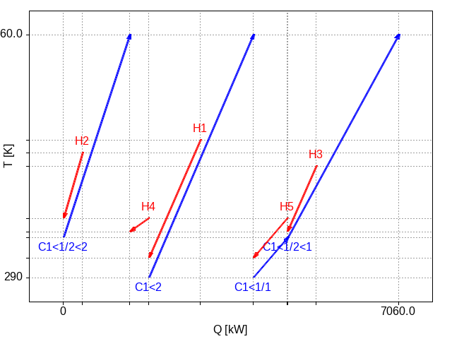
Figure 1: Plot of best solution found for Lewin's case study A.
Note: there is a bug in the generation of the png image for the plot in gnuplot which truncates the image too aggressively. The top label in the temperature (y) axis should be 660, the target temperature for stream C1.
The full details for the design of the heat exchanger network are summarised in this table:
| hot | Th,in | Th,out | cold | Tc,in | Tc,out | Duty | Area | Capital cost | Operating cost |
|---|---|---|---|---|---|---|---|---|---|
| K | K | K | K | kW | m2 | ||||
| H2 | 480.0 | 380.0 | C1<1/2<2 | 350.8 | 438.7 | 400.0 | 22.92 | 15489.56 | 0.00 |
| steam | 700.0 | 700.0 | C1<1/2<2 | 438.7 | 660.0 | 1006.0 | 12.33 | 12719.56 | 140842.70 |
| H4 | 380.0 | 360.0 | water | 300.0 | 320.0 | 400.0 | 11.40 | 12459.66 | 4000.00 |
| H1 | 500.0 | 320.0 | C1<2 | 290.0 | 472.4 | 1080.0 | 75.07 | 27046.11 | 0.00 |
| steam | 700.0 | 700.0 | C1<2 | 472.4 | 660.0 | 1110.6 | 14.83 | 13400.86 | 155477.82 |
| H5 | 380.0 | 320.0 | C1<1/1 | 290.0 | 349.6 | 720.0 | 47.69 | 21257.22 | 0.00 |
| H3 | 362.3 | 360.0 | C1<1/1 | 349.6 | 350.8 | 13.9 | 2.54 | 9709.14 | 0.00 |
| H3 | 460.0 | 362.3 | C1<1/2<1 | 350.8 | 428.6 | 586.1 | 59.06 | 23716.79 | 0.00 |
| steam | 700.0 | 700.0 | C1<1/2<1 | 428.6 | 660.0 | 1743.4 | 20.87 | 14974.87 | 244079.48 |
Post-processing would typically be applied to, for instance, combine the various pieces of stream C1 into a single stream to reach its target temperature using a single exchanger with hot utility. In principle, such a solution would be possible with the representation described above but is unlikely to be generated without a more intensive search in the design space. The above solution is found with only one thousand evaluations of F, the outer objective function. So, at most, one thousand configurations are considered.
Coming up
The next and probably final instalment of this series of blog posts will deal with the implementation of the Julia package that implements this bi-level optimization approach for heat exchanger network design. Watch this space!
Blog navigation
| Previous post | Blog | Next post |
|---|---|---|
| QTHEN: 3. Motivating stream splitting and cutting for heat exchanger network design | Index | QTHEN: 5. The QTHEN Julia package for heat exchanger network design |
You can find me on Mastodon or you can email me should you wish to comment on this entry or the whole blog.