The Fresa plant propagation algorithm for optimization
Table of Contents
- 1. Overview and introduction
- 2. Fresa – The code and documentation
- 2.1. start of module and dependencies
- 2.2. types
- 2.3. create a point deprecated
- 2.4. fitness
- 2.5. neighbour – generate random point
- 2.6. pareto – set of non-dominated points
- 2.7. printHistoryTrace - show history of a given solution
- 2.8. prune - control population diversity
- 2.9. randompopulation – for testing other methods
- 2.10. select – choose a member of the population
- 2.11. solve – use the PPA to solve the optimisation problem
- 2.12. thinout – make Pareto set smaller
- 2.13. utility functions
- 2.14. module end
- 3. Tests
- 4. Recent change history
- 5. Bibliography
| Author | Professor Eric S Fraga (e.fraga@ucl.ac.uk) |
| Version | 8.2.0 |
| Last revision | 2024-05-21 12:54:18 |
| Latest news | Support unbounded search domains and new fitness function. |
1. Overview and introduction
Fresa is an implementation of a plant propagation algorithm in Julia programming language. Our original version was called Strawberry, written in Octave (and usable in MATLAB). Please see the documentation of Strawberry for a longer description of the history of these codes, the conditions on which you may use these codes and which articles to cite. The quite interesting story of the strawberry plant can be found elsewhere.
The move to using Julia for the implementation of this algorithm was motivated by the desire to use open source and free (as in beer) software only while also ensuring that the tools are computationally efficient. Octave has not kept up with developments in just in time compilation and, although has some features not available in MATLAB, it is not a modern language. Julia provides many of the capabilities of Octave while also being computationally efficient and providing many more modern features such as built-in parallelism and multi-dispatch, both of which are used by Fresa for efficiency and to make the search procedure generic with respect to data types used to represent points in the search space.
A tutorial example, the design of the operating temperature profile for a simple reactor, modelled as a dynamic optimization problem, is available. A small example is presented below.
1.1. Licence and citing
All code (either version) is copyright © 2024, Eric S Fraga. See the LICENSE file for licensing information. Please note that the code is made available with no warranty or guarantee of any kind. Use at own risk. Feedback, including bug reports, is most welcome.
If either Fresa or Strawberry codes are used and this use leads to publications of any type, please do cite relevant sources. These include a short review article (Fraga 2021b),
@article{fresa-review-2021, author={Eric S. Fraga}, title={Fresa: A Plant Propagation Algorithm for Black-Box Single and Multiple Objective Optimization}, journal={International Journal on Engineering Technologies and Informatics}, year={2021}, volume={2}, number={4}, doi={} }
the software itself (Fraga 2021a),
@misc{fresa, author={Eric S. Fraga}, title={ericsfraga/Fresa.jl: First public release (r2021.06.30)}, journal={Zenodo}, note={{doi:10.5281/zenodo.5045812}}, year={2021}, doi={}, url={} }
and you may also wish to cite the original paper which led to the development of both Fresa and Strawberry, the first implementation of the plant propagation algorithm in MATLAB (Salhi and Fraga 2011):
@inproceedings{salhi-fraga-2011a,
  author={Abdellah Salhi and Eric S. Fraga},
  title={Nature-inspired optimisation approaches and the new plant propagation algorithm},
  booktitle={Proceedings of ICeMATH 2011, The International Conference on Numerical Analysis and Optimization},
  year={2011},
  pages={K2:1--8},
  address={Yogyakarta},
  month={6}
}
1.2. Support
For commercial and industrial users of this package, support is provided by Ananassa Consulting Ltd. Please email with your requirements.
1.3. Installation
This document has been written using org mode in the Emacs text editor. Org allows for literate programming and uses tangling to generate the actual source files for the code. The code, tangled from this file, can be found at github as a Julia package. Fresa has also been registered as a Julia package in the General registry. Therefore, all you should need to install Fresa is to type
add Fresa
in the Julia package manager, which you can activate by typing ] in the Julia REPL.
Fresa makes use of the following extra Julia packages: Dates, LinearAlgebra, Permutations, and Printf. These packages should be installed automatically by the Julia package manager if not already installed. The test problems below (and found in the test folder on github) may require one or more of the following extra packages: BenchmarkTools, PyPlot, Profile. You may need to install these explicitly to try out the test problems.
1.4. Quick example
Once Fresa is available in your Julia installation, using it requires you to define three aspects to define a problem:
- the objective function, including the evaluation of constraints if there are any;
- the search domain if the domain is bounded; and,
- an initial population, which can consist of a single point in the domain.
I will illustrate how to use Fresa for a simple nonlinear problem, adapted from chapter 13 of a textbook from MIT:1
![\[ \min_x z = 5 x_1^2 + 4 x_2^2 - 60 x_1 - 80 x_2 \]](ltximg/fresa_a3fe358d75c47566ae62ebd3204db34cffc7b5cd.png)
subject to the following constraints

and with ![\(x_1 \in [0,8]\)](ltximg/fresa_b294b5bc0638f4fdec2e5796b08b2826465ca197.png) and
and ![\(x_2 \in [0,\infty]\)](ltximg/fresa_b9fb3b54f82c91dfd74a24b5b0b4be7bcd4e06eb.png) .
.
We start by telling Julia that we wish to use the Fresa package:
using Fresa
The next step is to define the objective function. This function has two responsibilities: it must calculate the value of the objective and it must indicate whether the given point in the search space is feasible or not. The function returns a tuple consisting of z, the objective function value, and g, the indication of feasibility. g should be ≤ 0 if the point is feasible and greater than 0 otherwise. For constraints as in the example given above, the most straightforward approach can be to rewrite the constraints in the form  :
:

With this transformation, the objective function can be written:
function objective(x)
    # calculate the objective function value
    z = 5*x[1]^2 + 4*x[2]^2 - 60*x[1] - 80*x[2]
    # evaluate the constraints so that feasible points result in a
    # non-positive value, i.e. 0 or less, but infeasible points give a
    # positive value.  We choose the maximum of both constraints as
    # the value to return as an indication of feasibility
    g = max( 6*x[1] + 5*x[2] - 60,
             10*x[1] + 12*x[2] - 150 )
    # return the objective function value along with indication of
    # feasibility
    (z, g)
end
The second requirement is the definition of the search domain. For flexibility, for instance to allow the use of problem specific data structures, Fresa allows for the search domain to be a function of the search points. In that case, the domain would be defined by providing two functions, one which returns the lower bounds for the given point in the search space and the other returning the upper bounds. However, for problems with simple domains, involving a search in the real number domain, such as the example above, fixed lower and upper bounds can be defined. This is what we will do for this simple example.
In the problem definition above, the second optimization variable is unbounded in terms of the upper bound. However, looking at the constraints and taking into account the domain for the first optimization variable, we can determine that  must hold for feasible points. The search domain, for Fresa, is therefore defined as follows:
a = [ 0.0, 0.0 ]
b = [ 8.0, 12.5 ]
This code says that for any point in the search space, x, the lower bounds, a, are given by the vector [0.0, 0.0] and the upper bounds, b, by [8.0, 12.5]
Finally, an initial population must be provided to Fresa. This population can be of any size so long as there is at least one member. Fresa usually works well even if only one initial point in the search domain is provided. We consider starting at the midpoint of the search domain defined above and create a Point in the search domain:
initialpopulation = [ Fresa.Point( [4.0, 6.25 ], objective ) ]
Defining the Point object (see below) requires two arguments: the values of an actual instance of the decision or optimization variables in the search domain and the Julia function that evaluates the objective function for the optimization problem.
Given the above code, Fresa can now be used to solve the problem. The solve function has many options (see section 2.11 below) but these generally have reasonable defaults. The stopping criteria for the search include ngen for the number of generations and nfmax for the maximum number of objective function evaluations allowed. If neither is specified, the stopping criterion used is 100 generations.
best, population = Fresa.solve( objective,         # the function
                                initialpopulation, # initial points
                                lower = a,         # lower bounds
                                upper = b          # upper bounds
                                )
println("Population at end:")
println("$population")
println("Best solution found is:")
println("  f($( best.x ))=$( best.z )")
println("with constraint satisfaction (≤ 0) or violation (> 0):")
println("  g=$( best.g ).")
The arguments given here for the solve function are those that are required. There are also a number of optional arguments, as described in the code section below
If we execute all the above lines of code in Julia (see a Julia file with this code), the output will be similar to this:
# Fresa 🍓 PPA v8.2.0, last change [2024-04-04 14:40+0100]
* Fresa solve objective [2024-04-04 14:56]
#+name: objectivesettings
| variable | value |
|-
| elite | true |
| archive | false |
| ϵ | 0.0001 |
| fitness | scaled |
| issimilar | nothing |
| multithreading | false |
| nfmax | ∞ |
| ngen | 100 |
| np | 10 |
| nrmax | 5 |
| ns | 100 |
| steepness | 1.0 |
| tournamentsize | 2 |
|-
: function evaluations performed sequentially.
** initial population
#+name: objectiveinitial
|-
| z1 | g | x |
|-
| -503.75 | -4.75 | [4.0, 6.25] |
|-

** evolution
#+name: objectiveevolution
#+plot: ind:1 deps:(6) with:"points pt 7" set:"logscale x"
|       gen |       pop |        nf |    pruned |     t (s) | z1        |         g |
|-
|         1 |         1 |         1 |         0 |      2.09 | -503.75 | -4.75 |
|         2 |         3 |         3 |         0 |      3.13 | -503.75 | -4.75 |
|         3 |         6 |         8 |         0 |      3.13 | -505.54408373302675 | -4.358037407025066 |
|         4 |        17 |        24 |         0 |      3.13 | -505.54408373302675 | -4.358037407025066 |
|         5 |        31 |        54 |         0 |      3.13 | -505.54408373302675 | -4.358037407025066 |
|         6 |        30 |        83 |         0 |      3.13 | -511.5343571625019 | -3.218282063484118 |
|         7 |        28 |       110 |         0 |      3.13 | -511.5343571625019 | -3.218282063484118 |
|         8 |        31 |       140 |         0 |      3.13 | -513.9675221324901 | -2.4176768626883103 |
|         9 |        17 |       156 |         0 |      3.13 | -518.5612713991886 | -1.6236774582768803 |
|        10 |        29 |       184 |         0 |      3.13 | -519.8644456196524 | -1.3802989646061548 |
|        20 |        32 |       465 |         0 |      3.13 | -527.2735222717813 | -0.16509218562191563 |
|        30 |        30 |       746 |         0 |      3.13 | -528.8005114221052 | -0.01798427744348885 |
|        40 |        31 |      1022 |         0 |      3.13 | -529.2870222887932 | -0.07443020289168345 |
|        50 |        28 |      1291 |         0 |      3.13 | -529.6342609626806 | -0.020899244360016667 |
|        60 |        22 |      1545 |         0 |      3.13 | -529.7265340364295 | -0.0031986779201105264 |
|        70 |        33 |      1817 |         0 |      3.13 | -529.7265340364295 | -0.0031986779201105264 |
|        80 |        25 |      2085 |         0 |      3.13 | -529.7265340364295 | -0.0031986779201105264 |
|        90 |        33 |      2358 |         0 |      3.13 | -529.7265340364295 | -0.0031986779201105264 |
|       100 |        19 |      2646 |         0 |      3.13 | -529.7265340364295 | -0.0031986779201105264 |
** Fresa run finished
: nf=2675 npruned=0
Population at end:
|-
| z1 | g | x |
|-
| -529.7265340364295 | -0.0031986779201105264 | [3.6890324301409763, 7.572521348246806] |
| -490.2145940234657 | -1.2390932693507395 | [1.7760024502584146, 9.620978405819754] |
| -382.88238569370344 | 0.3433596773173164 | [0.0, 12.068671935463463] |
| -529.3515345351453 | -0.0958865900008945 | [3.6321759475721747, 7.6222115449132115] |
| -527.499895133928 | -0.5730366314000719 | [3.6301359737866523, 7.529229505176001] |
| -529.418653560424 | -0.0765247949718102 | [3.6254321522551587, 7.6341764582994465] |
| -529.2731002500146 | -0.11605337363324963 | [3.630202927642817, 7.62054581210197] |
| -530.6161764424138 | 0.22842496180827254 | [3.6843994395527813, 7.624405664898317] |
| -528.564871816406 | -0.3009321309140418 | [3.674385941400023, 7.530550444137164] |
| -527.9337546684199 | -0.4620345353414592 | [3.657980800461741, 7.518016132377619] |
| -527.2933472695051 | -0.5912770202773743 | [3.515757944734674, 7.662835062262916] |
| -527.0219720941407 | -0.6631082120947838 | [3.5149061362520113, 7.64949099407863] |
| -528.4621688329165 | -0.31095224816458256 | [3.5729267057945298, 7.650297503413649] |
| -530.3092023784462 | 0.1907812997138052 | [3.573312853808895, 7.750180835372086] |
| -527.809901442761 | -0.49295690026699646 | [3.6127958993500138, 7.5660535407265845] |
| -527.5470915135005 | -0.5481011542262308 | [3.5623499891604693, 7.615559782162191] |
| -526.0676154801108 | -0.9322132788217132 | [3.5792087212504895, 7.518506878735071] |
| -526.8382734769193 | -0.7398747868836182 | [3.619748619547411, 7.508326699166384] |
| -526.3991414268392 | -0.8499955992868848 | [3.612470819695875, 7.495035896507574] |
| -528.6884880504701 | -0.26917384925451415 | [3.6783282517648708, 7.532171328031252] |
| -527.5277495424356 | -0.5644041948620355 | [3.6540620444794927, 7.502244707652201] |
| -526.2072163725386 | -0.8978513187282573 | [3.6115084073935497, 7.486619647382089] |
| -528.7549881249026 | -0.2534750447939089 | [3.655903969983661, 7.562220227060826] |
| -529.1781613546334 | -0.13714804700559569 | [3.7208454323073643, 7.507555871830044] |
| -528.3891385783165 | -0.34216123656906916 | [3.6918799124114585, 7.5013118577924365] |
| -519.4967245902453 | 10.52859642940561 | [6.611892041465508, 6.171448836122515] |
| -529.831638289142 | 0.025243047617038883 | [3.659563338586391, 7.6135726032197395] |
| -530.050972250923 | 0.08292994187003444 | [3.7164801056479226, 7.5568098615965] |
| -529.620063048235 | -0.030761850076814312 | [3.66941272555407, 7.590552359319753] |
| -528.5002016045366 | -0.3149860430471989 | [3.6887883392372767, 7.510456784305827] |
|-

Best solution found is:
  f([3.6890324301409763, 7.572521348246806])=[-529.7265340364295]
with constraint satisfaction (≤ 0) or violation (> 0):
  g=-0.0031986779201105264.
The output includes details on the settings of all tunable parameters for the method (all of which can be adjusted, as noted above), the best solution in the population as it evolves, and the best in the final population along with that full population at the end. Note that the output is formatted to be best viewed using org mode2 in the Emacs3 text editor but the output should be readable as it is all just text.
A more complex tutorial example, the design of the operating temperature profile for a simple reactor, modelled as a dynamic optimization problem, is available. This example was the basis for a paper (Fraga 2019). It illustrates the generic nature of Fresa, allowing its application to problems with domain specific data structures. Note, however, that the code in that paper is based on version 7 of Fresa so some small changes would be required to have it work in version 8. See 1.6 section below for more details on the changes required in moving from version 7 to version 8.
1.5. Publications using Fresa
The following is a selection of publications which have been based on the use of Fresa and Strawberry:
- Optimization of a PID controller within a dynamic mdoel of a steam Rankine cycle with coupled energy storage (Ward et al. 2023).
- Discrete Formulation for Multi-objective Optimal Design of Produced Water Treatment (Falahi, Dua, and Fraga 2023)
- Multiple simultaneous solution representations in a population based evolutionary algorithm (Fraga 2021c).
- An example of multi-objective optimization for dynamic processes (Fraga 2019).
- Modelling of Microfluidic Devices for Analysis of Radionuclides (Pineda et al. 2019).
- Optimal design of hybrid energy systems incorporating stochastic renewable resources fluctuations (Amusat, Shearing, and Fraga 2018).
- On the application of a nature-inspired stochastic evolutionary algorithm to constrained multiobjective beer fermentation optimisation (Rodman, Fraga, and Gerogiorgis 2018).
1.6. Version information
- April 2024
- v8.2, minor release providing a number of upwards compatible enhancements including the following:
- support for fully unbounded search domains. See 2.5 section below for a description of the use of mapping from an unbounded domain to a bounded domain.
- addition of
:uniformfitness allocation method for single objective problems which is simply rank based fitness; the default is:scaledwhere the fitness is based on the objective function values. The default for multi-objective problems is:hadamardwhich is based on the product of the rankings for each objective. - the removal for the need to specify the measure of infeasibility for those problems where all points in the search domain are feasible. Objective functions can now simply return the value(s) of the objective(s).
- February 2024
- v8.1, minor release with improved control over output during the evolution of populations and added
lowerandupperbounds arguments as an alternative to thedomainargument. No breaking changes. - March 2023
- v8.0, major upgrade with possible breaking changes where I have refactored the calling sequences for some functions, specifically:
- Optional arguments to the main interface to Fresa, the
solvefunction, have changed:nfmaxhas been added as a second stopping criterion. Either this orngenis used to determine how much work to undertake in solving the problem. One of these must be set explicitly.ngendefaults to 100 unless eithernfmaxorngenis specified. This was the previous default but now a warning message is output if neither stopping criterion is specified.npophas been renamed tonpand stands for the number of solutions to propagate in each generation. It is not the size of the population.tolerancehas been renamed toϵand is used by the next change:The pruning of the population is now controlled by a new optional argument,
issimilar, which expects to be set to the name of a function which compares two points and returntrueif the two points should be considered similar. If this function is defined, and if the optional argumentϵis set to a value greater than 0 (default value is 0.0001), then pruning will take place. The default value forissimilarisnothingso pruning is turned off by default. Example functions suitable for assignment toissimilarare given below.The signature of the
issimilarfunction is:function issimilar( p1::Point, p2::Point, ϵ::Float64, domain::Domain)
and two useful implementations, for real valued decision variables and real valued objective function values, are provided:
Fresa.similarxandFresa.similarz.
- deprecated the
createpointfunction and use thePointstructure constructor directly.createpointis still available so this is not a breaking change although it is recommended that any call tocreatepointbe replaced with the instantiation of aFresa.Pointdata type directly. Removed the need to pass a
Domainobject to theneighbourfunction as there are problems which are unbounded or for which the bounds are implicitly encoded in the decision variables. This is a breaking change firstly because thesolvefunction arguments have changed so that thedomainis now an optional parameter as opposed to a required argument. Secondly, for problem specificneighbourfunctions, the order of the arguments has changed to cater for the domain being an optional argument to thesolvefunction. Specific details follow on how to update any version 7 code to version 8.To update any code that worked with version 7 to now work with version 8, the key change is the call to the
solvemethod. Previously, the call would have been in the formFresa.solve(f, p0, domain, ...)
where
...indicates optional parameters. This call would need to be changed toFresa.solve(f, p0, domain = domain, ...)
Further, any definition of an application specific
neighbourfunction would be changed from having an argument listFresa.neighbour(x, a, b, f)
where
aandbdefined lower and upper bounds for the search domain, in version 7, would now beFresa.neighbour(x, f, domain)
with
domainbeing an instance of theFresa.Domaindata type. The lower and upper bounds can be obtained bya = domain.lower(x) b = domain.upper(x)
in the
neighbourfunction.For problems where the domain is not required or useful, this
domainargument is optional and the signature of an application specificneighbourmethod may beFresa.neighbour(x, f)
where the call to the
solvemethod can simply not provide aDomainargument if it is not necessary for identifying valid neighbouring solutions.
- Optional arguments to the main interface to Fresa, the
- February 2023
- minor update to version 7.2.42 prior to the release of a new major version.
- June 2021
- v7.2.1, first public release via github and Zenodo: 10.5281/zenodo.5045812 (Fraga 2021a).
- May 2021
- v7.1, implemented multithreading in the evaluation of the population for each generation. This introduces a new option for the
solvemethod:multithreadingwhich can be set to eithertrueorfalsewith the latter being the default. Julia must be invoked with the--threadsargument (or-tfor short) with the number of threads to use orautofor automatic determination of the threads possible. Multithreading is useful when the evaluation of the objective function is computationally expensive. Otherwise, the overhead of multithreading is usually not worth it although it is not detrimental. - April 2021
- v7,
- the domain for the search, which has to be bounded, is now defined by a
Domaindata structure which allows for different representations of solutions in the search space in a given population; - allow setting the steepness of the fitness adjustment function. This is an outcome of the presentation by Wouter Vrielink at the PPA mini-zoomposium I organised in March 2021 to discuss the impact of PPA parameters on the effectiveness of the search procedure.
- the domain for the search, which has to be bounded, is now defined by a
- March 2021
- v6, one of the required arguments to the
solvefunction has been changed. Specifically, the initial guess must now be a population ofPointobjects and not a single decision variable. See examples below for how to create this initial population easily. - April 2020
- moved all code to github. This should make it easier for others to use the code.
- September 2019
- v5, The objective function values, in the
Pointtype, are now a genericVectorinstead of an array of floating point numbers. This opens up Fresa to be used for objective functions which are not necessarily simple scalar values. The use case has been illustrated through a case study in stochastic optimization, specifically design under uncertainty. Details available from the author. - July 2019
- v4, The returned values for
Fresa.solvein the single objective case have changed. Instead of separate returned values for the decision variables, the objective function value, etc., a singleFresa.Pointvalue is returned for the best point found, along with the full final population as an array ofFresa.pointvalues. - June 2019
- v3, The calling interface for using the
Fresa.solvemethod has changed. Specifically, when the search space is defined by data structures that are not a vector ofFloat64values, the user must create aFresa.neighbourfunction definition for the specific data structure type. - September 2017
- v2, moved to an object representation for points in the search space and allowed for parallel evaluation of the objective function when multiple processors are available.
- November 2016
- v1, first Julia plant propagation algorithm implementation.
A list summary of recent change history is given below.
2. Fresa – The code and documentation
The Fresa method is a population based evolutionary algorithm which mimics the propagation used by plants. Throughout the module, the population object is an array of Point objects. Each point is defined by the decision or optimization variables (the point in a search space), the objective function values for this point and a feasibility indication, with g≤0 feasible and g>0 infeasible. See the documentation for the solve method below for more details on the data structures used and expected.
2.1. start of module and dependencies
Fresa depends on a number of packages that should be available in any Julia installation. These are packages for mostly for displaying output formatted for easy viewing in the Emacs text editor using org mode.
# All code copyright © Eric S Fraga.
# Licence for use and sharing can be found at
#   https://github.com/ericsfraga/Fresa.jl/blob/master/LICENSE
# Date of last change in version variable below.
module Fresa
version = "8.2.0"
lastchange = "[2024-05-21 12:54+0100]"
using Dates                     # for org mode dates
using LinearAlgebra             # for norm function
using Permutations              # for random permutations of vectors
using Printf                    # for formatted output
function __init__()
    println("# Fresa 🍓 PPA v$version, last change $lastchange")
end
2.2. types
2.2.1. Point
Fresa uses one type, Point, which is a point in the search space. It includes these entries:
x- of indeterminate type to allow for a wide range of applications (e.g. integer versus real values),
z- the value of the objective function, as a vector, where the entries in the vector can be of any type that can be compared and sorted by
sortperm4 or, in the case of multiple criteria, where it can be determined whether one point dominates another, g- the constraint violation (feasible with ≤0 and infeasible otherwise) always of type
Float64(for now), and ancestor- another point in the search space, along with some extra information, that led to the creation of this point.
An instance of a point is defined by the variable in the search space, the objective function used to evaluate the point, the ancestor of this point (see below), and optional parameters to pass to that function.
As Fresa is an evolutionary procedure, every point in the search space considered will be the descendent of a previously considered point. The sole exception is the initial starting point given by the procedure which invokes Fresa. The link between points is through a backward chain defined by the ancestor entry. This is not used by Fresa itself directly but provides extra meta-information that could be useful for post-optimization analysis, e.g. to see how effective the balance between exploration and exploitation may be for the given search parameter values.
An issue in Julia (as of 2021, at least) is that you cannot define two data structures that mutually refer to each other. Therefore, the type of the ancestor entry in the Point data structure has to be defined later (see Ancestor definition below). This is discussed in the issue for Julia on github.
"""

Point (`x`) in the search space along with objective function values
(`z[]`) and feasbility indication (`g`).  The type of `x` is problem
specific.  `z[]` and `g` hold `Float64` values.  `g` should be of
length 1.

When evaluating the objective function, `f` in the constructor, the
value returned will be a `Tuple` if both the objective function value
and the measure of infeasibility are specified.  If a tuple is not
returned, the return value will be taken to be the objective function
value and the feasibility measure will be assumed to be 0.0, i.e. a
feasible point in the search domain.

"""
struct Point
    x :: Any                    # decision point
    z :: Vector                 # objective function values
    g :: Float64                # constraint violation
    ancestor                    # the parent of this point
    function Point(x,           # point in search space
                   f,           # objective function
                   parameters = nothing, # arguments to objective function
                   ancestor = nothing)   # for analysis of search process

        # evaluate the objective function.  The parameters are passed
        # to the function if defined, i.e. not Nothing.  The returned
        # value will either be a tuple consisting of the objective
        # function value and the measure of infeasibility or it will
        # be just the objective function value alone with an implied
        # zero value for the infeasibility measure.
        ret = parameters isa Nothing ? f(x) : f(x, parameters)
        # pick out the objective function value and measure of
        # infeasibility from the returned value
        z, g = ret isa Tuple ? ret : (ret, 0.0)

        if g isa Int
            g = float(g)
        end

        # now create the actual Point object, ensuring that the
        # objective function value is always a vector, even for single
        # objective function problems.
        p = Nothing
        if rank(z) == 1
            p = new(x, z, g, ancestor)
        elseif rank(z) == 0
            p = new(x, [z], g, ancestor)
        else
            error("Fresa can only handle scalar and vector criteria, not $(typeof(z)).")
        end
        return p
    end
end
Customise how a Point is displayed. We display the objective function value(s) first and then the representation of the point. This allows for a population to have different representations without causing problems with any data analysis on the columns representing the objective function values.
import Base
Base.show(io::IO, p::Fresa.Point) = print(io, "f(", p.x, ")=", p.z, " g=", p.g)
# and also an array of points
function Base.show(io::IO, p::Array{Point,1})
    np = length(p)
    if np > 0
        nz = length(p[1].z)
        println(io, "|-")
        for i=1:nz
            print(io,"| z$(i) ")
        end
        println(io, "| g | x |")
        println(io,"|-")
        for i=1:length(p)
            for j=1:nz
                print(io,"| ", p[i].z[j], " ")
            end
            print(io, "| ", p[i].g, " ")
            print(io, "| ", p[i].x, " |\n")
        end
        println(io,"|-")
    else
        print(io,"empty")
    end
end
and also indicate that a Point is atomic in a sense:
import Base.size
Base.size(p :: Point) = ()
2.2.2. Ancestor
The creation of any point in the search is based on one of the existing points in the population. This existing point is known as the ancestor of the new point. The Ancestor data structure is used to connect points to their ancestors and collect information about when and how the new point was created.
struct Ancestor
    point :: Point        # the actual ancestor point
    fitness :: Float64    # the fitness of the ancestor
    generation :: Int32   # the generation when this point was created
end
Once the Ancestor data structure has been defined, we can now use an access constructor to define the type for the ancestor field in the Point object:
ancestor(p :: Point) = p.ancestor :: Union{Ancestor,Nothing}
2.2.3. Domain
Fresa assumes a bounded domain for the search. Each design variable will have a lower and upper bound. To provide for domain specific design variable data structures, the Domain structure is used. In this structure, the lower and upper variables are functions which will be evaluated with a point in the search space and are expected to return appropriate data that the neighbour function (see below) will be able to use to ensure the domain bounds are respected in the creation of new search points.
struct Domain
    lower                       # function which returns lower bound on search variable(s)
    upper                       # function which returns upper bound on search variable(s)
end
An example of a the use of this Domain structure is:
d = Fresa.Domain(x -> zeros(length(x)), x -> ones(length(x)))
which will define the domain as a unit square, ![\(x \in [0,1]^n\)](ltximg/fresa_c1c8883cb921af3b7b89f62456421bcd257635f6.png) , as defined by the size of the
, as defined by the size of the x argument.
2.3. create a point deprecated
A trivial function that simply creates a new Point object. This exists for two reasons:
- It is needed for the
remotecallfunctionality when using parallel computing because theremotecallfunction has to be given a function and not just a constructor (for some obscure reason that means that a constructor is transformed to a conversion operation… don't ask me). - The
Pointtype is parametric. This makes defining a generic constructor difficult (at least, I was unable to find a working solution).
The optional parameters and ancestor arguments are passed through to their respective destinations: the objective function for the parameters and the point creation for the ancestor linking.
function createpoint(x,f,parameters = nothing,ancestor = nothing)
    z = 0
    g = 0
    if ! ( parameters isa Nothing )
        (z, g) = f(x, parameters)
    else
        (z, g) = f(x)
    end
    if g isa Int
        g = float(g)
    end
    p = Nothing
    if rank(z) == 1
        p = Point(x, z, g, ancestor)
    elseif rank(z) == 0
        p = Point(x, [z], g, ancestor)
    else
        error("Fresa can only handle scalar and vector criteria, not $(typeof(z)).")
    end
    return p
end
(deprecated) and we provide two versions with simple calling sequences:
function createpoint(x,f)
    return createpoint(x,f,nothing,nothing)
end
function createpoint(x,f,parameters)
    return createpoint(x,f,parameters,nothing)
end
2.4. fitness
The fitness function used depends on the number of objectives. For single criterion problems, the fitness is the objective function values normalised and reversed so that the minimum, i.e. the best solution, has a fitness of close to 1 and the worst a fitness close to 0. For multi-criteria problems, a Hadamard product of individual criteria rankings is used to create a fitness value (Fraga & Amusat, 2016) with the same properties: best solutions have fitness values closer to 1 than less fit solutions.
This function uses a helper function, defined below, to assign a fitness to a vector of objective function values.
function fitness(pop, fitnesstype, steepness, generation, ngen)
    l = length(pop)
    indexfeasible = (1:l)[map(p->p.g,pop) .<= 0]
    indexinfeasible = (1:l)[map(p->p.g,pop) .> 0]
    @debug "Feasible/infeasible breakdown" indexfeasible indexinfeasible maxlog=3
    fit = zeros(l)
    factor = 1              # for placement in fitness interval (0,1)
    if length(indexfeasible) > 0
        feasible = view(pop,indexfeasible)
        # use objective function value(s) for ranking
        feasiblefit = vectorfitness(map(p->p.z,feasible), fitnesstype, steepness, generation, ngen)
        if length(indexinfeasible) > 0
            feasiblefit = feasiblefit./2 .+ 0.5 # upper half of fitness interval
            factor = 2                        # have both feasible & infeasible
        end
        fit[indexfeasible] = (feasiblefit.+factor.-1)./factor
    end
    if length(indexinfeasible) > 0
        # squeeze infeasible fitness values into (0,0.5) or (0,1) depending
        # on factor, i.e. whether there are any feasible solutions as well or not
        infeasible = view(pop,indexinfeasible)
        # use constraint violation for ranking as objective function values
        # may not make any sense given that points are infeasible
        fit[indexinfeasible] = vectorfitness(map(p->p.g, infeasible),
                                             fitnesstype,
                                             steepness,
                                             generation,
                                             ngen
                                             ) / factor;
    end
    fit
end
The helper function works with a single vector of objective function values which may consist of single or multiple objectives.
"""
For single objective problems, the fitness is simply the normalised
objective function value.

For multi-objective cases, there are three alternative measures of
fitness ranking possible.  The first is based on the Hadamard product
of the rank of each member of population accoring to each
criterion.  The second is based on a weighted Borda ranking based on
each criterion ranking.  Finally, a measure based on dominance,
similar to that used by the popular NSGA-II genetic algorithm, is
available.

"""
function vectorfitness(v, fitnesstype, steepness, generation, ngen)
    # determine number of objectives (or pseudo-objectives) to consider in
    # ranking
    l = length(v)
    if l == 1
        # no point in doing much as there is only one solution
        fit = [0.5]
    else
        m = length(v[1])
        # println("VF: v=$v")
        # println("  : of size $(size(v))")

        # treat single objective and multi-objective fitness
        # calculations differently.  The latter is more complex due to
        # the concept of non-domination and solutions having
        # equivalent "goodness" despite different objective function
        # values.
        if m == 1
            # if there is only one objective function value, the
            # fitness is simply based on the value of this objective
            # function, noting that the assumption is that the
            # optimization problem is one of minimization.  There are
            # two types of fitness assignment for this case: a fitness
            # based on the relative values of the objective function
            # and a fitness assignment that is uniform in the [0,1]
            # interval.
            if fitnesstype == :scaled
                fitness = [v[i][1] for i=1:l]
            elseif fitnesstype == :uniform
                fitness = ones(l)
                fitness[sortperm([v[i][1] for i=1:l])] = 1:l
            end
        else                  # multi-objective
            rank = ones(m,l); #rank of each solution for each objective function
            if fitnesstype == :hadamard
                for i=1:m
                    rank[i,sortperm([v[j][i] for j=1:l])] = 1:l
                end
                # hadamard product of ranks
                fitness = map(x->prod(x), rank[:,i] for i=1:l)
            elseif fitnesstype == :borda
                for i=1:m
                    rank[i,sortperm([v[j][i] for j=1:l])] = 1:l
                end
                # borda sum of ranks
                fitness = map(x->sum(x), rank[:,i] for i=1:l)
            elseif fitnesstype == :nondominated
                # similar to that used by NSGA-II (Deb 2000)
                fitness = zeros(l)
                maxl = assigndominancefitness!(fitness,v,1)
                # println("Resulting fitness: $fitness")
            else
                throw(ArgumentError("Type of fitness evaluation must be either :borda, :nondominated, or :hadamard, not $(repr(fitnesstype))."))
            end
        end
        # normalise (1=best, 0=worst) while avoiding
        # extreme 0,1 values using the hyperbolic tangent
        fit = adjustfitness(fitness, steepness, generation, ngen)
        # println(":  scaled fitness: $fit")
        @debug "Fitness calculations" v[1][1] v[2][1] v[l][1] fitness[1] fitness[2] fitness[l] fit[1] fit[2] fit[l] maxlog=3
    end
    fit
end
The fitness should be a value ∈ (0,1), i.e. not including the bounds themselves as those values cause some silly behaviour in the definition of individual neighbouring solutions (i.e. the runners) and the number of runners. Therefore, we adjust the fitness values to ensure that the bounds are not included.
See below for a discussion about the second function argument, steepness, and how the value s is calculated if steepness is a tuple and not a single value.
function adjustfitness(fitness, steepness, generation, ngen)
    if (maximum(fitness)-minimum(fitness)) > eps()
        s = steepness
        if steepness isa Tuple
            a = (2*steepness[1]-2*steepness[2])/3
            b = - (3*steepness[1] - 3*steepness[2])/ngen^2
            d = steepness[1]
            s = a*generation^3 + b*generation^2 + c*generation + d
            @debug "Steepness " s "at generation" g
        end
        fit = 0.5*(tanh.(4*s*(maximum(fitness) .- fitness)
                         / (maximum(fitness)-minimum(fitness))
                         .- 2*s) .+ 1)
    else
        # only one solution (or all solutions the same) in population
        fit = 0.5*ones(length(fitness))
    end
    fit
end
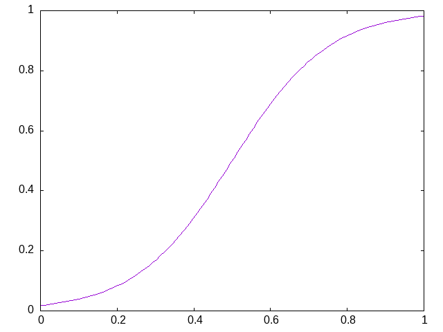
This function takes, as an argument, the steepness of the transition from poor fitness to good fitness. Some plots are useful for comparison. This first plot shows the default fitness adjustment function which gives some emphasis to the extreme values but also ensures that the fitness values are quite some distance from the boundary of the fitness domain:
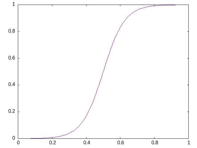
Making the fitness adjustment steeper, e.g. with a value of steepness of 2 instead of the default value of 1, the function has a more pronounced emphasis towards the boundaries and allows values closer to those boundaries:
The steepness may be specified as a tuple in which case it represents the initial value for the steepness and the final value. The evolution of the steepness is based on a cubic with 0 slope at the start and at the end. The following maxima code is the solution of the that cubic given the need to pass through the points  and
and  where
where  and
and  are the two values of the tuple and
  is the number of generations:
c(g) := a*g^3 + b*g^2 + c*g + d;
define(d(g), diff(c(g),g));
equations: [c(0) = s1,
d(0) = 0,
c(n) = s2,
d(n) = 0];
solution: solve(equations, [a, b, c, d]);
for i: 1 thru length(solution[1]) do print(solution[1][i])$
    2 s1 - 2 s2
a = -----------
         3
        n
      3 s1 - 3 s2
b = - -----------
           2
          n
c = 0
d = s1
The following function is used by the vector fitness evaluation to recurse through the levels of non-dominance to assign fitness based on those levels.
function assigndominancefitness!(f,v,l)
    # assign value l to all members of v which dominate rest and then
    # recurse on those which are dominated
    (p, d) = paretoindices(v)
    # println("Assigning fitness $l to $p")
    f[p] .= l
    if !isempty(d)
        assigndominancefitness!(view(f,d),v[d],l+1)
    else
        l
    end
end
2.5. neighbour – generate random point
A random solution is generated with a distance from the original point being inversely proportional, in a stochastic sense, to the fitness of the solution. The new point is possibly adjusted to ensure it lies within the domain defined by the lower and upper bounds. The final argument is the fitness vector with values between 0 and 1, 1 being the most fit and 0 the least fit.
Fresa comes with two default methods for generating neighbouring solutions.
2.5.1. Floating point decision variables
- vector of floating point numbers
The first is for a search space defined by vectors of
Float64values:function neighbour(x :: Vector{T}, f :: Float64, d :: Domain ) :: Vector{T} where T <: AbstractFloat # allow movements both up and down in the domain for this variable # so determine the actual domain lower and upper bounds a = d.lower(x) b = d.upper(x) xnew = x .+ (1.0 .- f) .* 2(rand(length(x)).-0.5) .* (b.-a) xnew[xnew.<a] = a[xnew.<a]; xnew[xnew.>b] = b[xnew.>b]; return xnew end
- single floating point number
There is also a version that expects single valued
Float64arguments.function neighbour(x :: Float64, f :: Float64, d :: Domain ) :: Float64 # allow movements both up and down # in the domain for this variable a = d.lower(x) b = d.upper(x) newx = x + (b-a)*(2*rand()-1)/2.0 * (1-f) if newx < a newx = a elseif newx > b newx = b end newx end
Should other decision point types be required, e.g. mixed-integer or domain specific data structures, the
Fresa.neighbourfunction with parameters of the specific type will need to be defined. See the mixed integer nonlinear examples below for an example of a simple mixed-integer case. - unbounded search domain for vectors of floating point numbers
In v8.2, we have introduced the capability of searching within an unbounded domain. The approach taken is to map the unbounded domain, (-∞,+∞), to a bounded domain, (-π/2,+π/2), using the
atanandtanfunctions to go from the unbounded domain to a bounded domain and vice versa, respectively. This is the approach used by Chow, Tsui, and Lee (2001) and Ishizawa et al. (2023) propose another method and give a short summary of alternatives.An unbounded domain is identified by having an undefined
domainargument to theneighbourfunction, as implemented here. Adaptations of theneighbourfunction for problems involving something other than vectors of floating point numbers for the decision variables would have to be modified accordingly to handle unbounded search domains.function neighbour(x :: Vector{Float64}, f :: Float64 ) :: Vector{Float64} # map given point to the domain (-π/2,+π/2) x̂ = atan.(x) # and define the bounds on the mapped space a = (-π/2+eps())*ones(length(x)) b = (+π/2+eps())*ones(length(x)) xnew = x̂ .+ (1.0 .- f) .* 2(rand(length(x)).-0.5) .* (b.-a) xnew[xnew.<a] = a[xnew.<a]; xnew[xnew.>b] = b[xnew.>b]; return tan.(xnew) end
2.5.2. Integer decision variables
- vector of integer values including binary variables
function Fresa.neighbour(y :: Vector{Int},
                         ϕ :: Float64,
                         d :: Fresa.Domain)
    # do not overwrite the argument
    ret = copy(y)
    n = length(y)
    # get lower and upper bounds
    a = d.lower(y)
    b = d.upper(y)
    # determine the order in which variables are chosen
    ind = RandomPermutation(n).data
    # choose how many to adjust
    na = Int(ceil((1.0-ϕ)*rand()*n))
    @assert na ≤ n
    for i ∈ 1:na
        # consider the case of binary variables as special cases:
        # toggle the boolean value (which is essentially what a binary
        # variable can be considered to be); otherwise, change value
        # up or down randomly.
        if a[i] == 0 && b[i] == 1
            # binary variable
            ret[i] = 1 - ret[i]
        else
            # determine direction to adjust the integer value
            dir = rand([-1, 1])
            # check to make sure we can move in that direction
            if (ret[ind[i]]+dir) < a[ind[i]] || (ret[ind[i]]+dir) > b[ind[i]]
                dir = -dir
            end
            # and then move a random distance based on how far from
            # the bounds the current value is
            delta = rand() * (1.0-ϕ) *
                ((dir < 0) ? (ret[ind[i]]-a[ind[i]]) : (b[ind[i]]-ret[ind[i]]))
            ret[ind[i]] = ret[ind[i]] + dir*ceil(delta)
        end
    end
    return ret
end
2.6. pareto – set of non-dominated points
Select a set consisting of those solutions in a population that are not dominated. This only applies to multi-objective optimisation; for a single criterion problem, the solution with minimum objective function value would be selected. This function is used only for returning the set of non-dominated solutions at the end of the solution procedure for multi-objective problems. It could be used for an alternative fitness function, a la Srinivas et al. (N Srinivas & K Deb (1995), Evolutionary Computation 2:221-248).
2.6.1. dominates: determine dominance
To cater for generic comparisons between points in the objective function space (e.g. distributions instead of single values for each objective function), we introduce an operator used to determine dominance. The community differs on the symbol to use for dominates. Some5 use ≼ (\preceq); others6 use ≻ (\succ). I have decide to use the latter as it gives the impression of dominating.
function dominates(a, b)
    all(a .<= b) && any(a .< b)
end
≻(a,b) = dominates(a,b)
This operator will be extended by other packages that wish to make comparisons between non-scalar values of each objective function. The easiest way may often be to ensure that ≤ and < operators are defined for the individual entries in the vector of objective function values.
2.6.2. find Pareto set
The following code splits a population into those points that are non-dominated (i.e. would be considered an approximation to a Pareto frontier) and those that are dominated. The function returns indices into the population passed to it.
function paretoindices(z)
    n = length(z)
    dominance = [reduce(&, [!(z[i] ≻ z[j]) for i ∈ 1:n]) for j ∈ 1:n]
    paretoindices = filter(j -> dominance[j], 1:n)
    dominatedindices = filter(j -> !dominance[j], 1:n)
    (paretoindices, dominatedindices)
end
Given a population of Point objects, this function identifies those that are non-dominated (see above). If the population includes both feasible and infeasible points, only those that are feasible are considered.
# indices of non-dominated and dominated points from the population of
# Point objects
function pareto(pop :: Vector{Point})
    l = length(pop)
    indexfeasible = (1:l)[map(p->p.g,pop) .<= 0]
    indexinfeasible = (1:l)[map(p->p.g,pop) .> 0]
    if length(indexfeasible) > 0
        subset = view(pop,indexfeasible)
        indices = indexfeasible
    else
        #println(": Fresa.pareto warning: no feasible solutions.  Pareto set meaningless?")
        subset = pop
        indices = 1:l
    end
    z = map(p->p.z, subset)
    # use function below to return indices of non-dominated and
    # dominated from objective function values alone in the subset of
    # feasible solutions
    (p, d) = paretoindices(z)
    (indices[p], indices[d])
end
2.7. printHistoryTrace - show history of a given solution
Each point encountered in the search, other than points in the initial population, is the result of propagating another point. When a new point is created, a link back to its parent point is created. This allows us to explore the history of all points in the search. This function prints out the historical trace of a given point, using an org table for formatting.
function printHistoryTrace(p :: Point)
    a = p.ancestor
    while ! (a isa Nothing)
        println("| $(a.generation) | $(a.fitness) |")
        a = a.point.ancestor
    end
end
2.8. prune - control population diversity
Due to the stochastic nature of the method and also the likely duplication of points when elitism is used, there is often or at least sometimes the need to prune the population. If a function, issimilar, has been provided that defines a measure of similarity, this function is applied to pairs of points in the search, including their objective function values, to identify similar solutions and remove them from the population. The similarity can make use of a tolerance, ϵ.
The issimilar function can define similarity based on the decision variables, the objective function values, or a combination of the two. Two functions are provided below, one for decision variables and one for objective function values.
function prune(pop :: AbstractArray, issimilar, ϵ, domain)
    l = length(pop)
    # we will return a diverse population where similar solutions have
    # been removed
    diverse = [pop[1]]
    # consider each solution in the population
    for i=2:l
        similar = false
        j = 0
        # compare this solution with all already identified as diverse
        # enough
        while !similar && j < length(diverse)
            j += 1
            similar = issimilar(diverse[j], pop[i], ϵ, domain)
        end
        if !similar
            push!(diverse,pop[i])
        end
    end
    # return diverse population and count of points removed
    (diverse, length(pop)-length(diverse))
end
2.8.1. similarx
A function that compares solutions based on the decision variables, where these variables are suitable for the difference operator, -, and that the LinearAlgebra.norm function can accept this difference as an argument. For other decision variables, e.g. a complex data type, a new similarity function will have to be defined.
To avoid considering two solutions that straddle a constraint boundary, i.e. one feasible and the other infeasible, the constraint violation, g, is also considered even though the objective function values are not.
Arguments: p1 and p2 are two points in the search space to compare and ϵ>0 the tolerance for similarity.
function similarx(p1, p2, ϵ, domain)
    norm(p1.x-p2.x) < ϵ &&      # decision variables
        norm(p1.g-p2.g) < ϵ &&  # difference in violation
        ( (p1.g ≤ 0 && p2.g ≤ 0) || (p1.g > 0 && p2.g > 0)) # both same feasibility
end
As this similarity function compares decision variables, the domain could be used to compare solutions for a relative difference based on the size of the domain. This is left as an exercise for the reader.
2.8.2. similarz
A function that compares solutions based on objective function values, z, and returns true if the two points passed are considered to be similar, enough that the search would benefit from not having both present in the population in terms of diversity. This really only makes sense for an objective function space that is unimodal. The more appropriate similarity test for multimodal objective function spaces would be comparing on the decision variables (see above).
Again, the constraint violation, g, is taken into consideration in identifying similar solutions.
Arguments: p1 and p2 are two points in the search space to compare and ϵ>0 the tolerance for similarity.
function similarz(p1, p2, ϵ, domain)
    norm(p1.z-p2.z) < ϵ &&      # objective function values
        norm(p1.g-p2.g) < ϵ &&  # difference in violation
        ( (p1.g ≤ 0 && p2.g ≤ 0) || (p1.g > 0 && p2.g > 0)) # both same feasibility
end
2.9. randompopulation – for testing other methods
Create a random population of size n evaluated using f. A single point, x, in the search domain must be given as the domain definition is function based and the lower and upper bounds are potentially a function of the location in the space. The randompoint method below is suitable for domains defined by float valued vectors.
function randompopulation(n, f, parameters, p0, domain :: Domain)
    p = Point[]                 # population object
    for j in 1:n
        # l = domain.lower(p0.x)
        # @show l
        # u = domain.upper(p0.x)
        # @show u
        # x = randompoint(l,u)
        # push!(p, createpoint(x, f, parameters))
        push!(p, Point(randompoint(domain.lower(p0.x), domain.upper(p0.x)),
                       f, parameters))
    end
    p
end
By default, the following method generates a random point within the search domain. This does not attempt to find a feasible point, simply one within the box defined by lower, a, and upper, b, bounds.
# for single values
function randompoint(a :: Float64, b :: Float64)
    x = a + rand()*(b-a)
end
# and for vectors of values (which could in principle be integer
# values)
function randompoint(a, b)
    x = a + rand(length(a)).*(b-a)
end
2.10. select – choose a member of the population
Given a fitness, f, choose two solutions randomly and select the one with the better fitness. This is known as a tournament selection procedure with the given size, which defaults to 2 in the solve function unless given a value by caller of that function. Other select methods are possible but not currently implemented.
function select(f, size)
    indices = rand(1:length(f), size)       # generate size indices
    best = argmax([f[i] for i ∈ indices])
    indices[best]
end
2.11. solve – use the PPA to solve the optimisation problem
The solve function is the main (only) entry point for the Fresa optimization package. The following details all the arguments, both required and optional, for this function:
Required arguments:
- f
objective function.
The calling sequence for
fis a point in the search space plus, optionally, theparametersdefined in the call tosolve(see optional arguments below).The objective function should return a tuple consisting of two entries: the first is the objective function value(s), which must be either a scalar real value or a vector of real values, and the second a value giving the the constraint violation. If
g≤0, the point is considered to have satisfied all constraints for the optimization problem and hence is feasible. Ifg>0, at least one constraint has been found to not be satisfied so the point is infeasible. The value ofgfor infeasible points will be used to rank the fitness of the infeasible solution, with lower values being fitter, i.e. more close to being feasible.See the simple example in the introduction to Fresa.
- p0
- initial population with at least one initial point in the search space but there can be any number of points defined intially. There is no requirement that all the points be based on the same data structure for the decision variables. See the 2.5 function for details and the use of multiple dispatch to enable heterogeneous populations in the search procedure (Fraga 2021c).
Optional arguments:
- archiveelite
- save thinned out elite members; default value
false. When solving multi-objective problems, the elite set in a population is defined by the set of non-dominated points. This set of points can grow too large and end up dominating (no pun intended) the population. For this reason, if the set of non-dominated points grows beyond half of the population, this set will be trimmed. Ifarchiveeliteis set totrue, the members trimmed will be added to an archive and this archive will be updated every generation. The archive will be added to the final population at the end of the search. - domain
- search domain: will often be required but not always; default value
nothing. The domain, if given, will be passed to the 2.5 function which will allow neighbour generation to know about the search domain. The domain, if defined, must be a Domain object. Alternatively, thelowerandupperbounds can be specified and aDomainobject will be created from these. The possibility of defining theDomainobject directly is that it allows for dynamic domains and domains that depend on the current point in the search space. See this paper for an example of how this can be used to support multiple simultaneous alternative representations of solutions and hence search spaces. - elite
- elitism by default; default value
true. The elite member (single objective problem) or members (set of non-dominated points for multi-objective problems) will automatically be part of the next generation's population if this istrue. This avoids the problem with stochastic methods which identify a good solution but then lose it because of a stochastic selection mechanism. However, the disadvantage of elitism is that it can lead to premature convergence to a sub-optimal solution. - ϵ
- ϵ for similarity detection; default value 0.0001. This will be passed to the
issimilarfunction if diversity control is desired. - fitnesstype
- how to rank solutions in multi-objective case; default value
:hadamard. The following options are available for this argument:- :borda
- assigns fitness according to the Borda sum of the individual points ranked according to each criterion independently. Similar to the
:hadamarddefault. - :hadamard
- assigns fitness according to the Hadamard product of the individual rankings with respect to each criterion (Fraga and Amusat 2016).
- :nondominated
- uses a sorting algorithm proposed by Deb (Deb 2000);
- issimilar
- function for diversity check: see No description for this link function; default value
nothing. If this function is defined, andϵ>0, the function specified will be invoked with pairs of points to identify those which are similar and could be removed from the population to ensure diversity is maintained. Two pre-defined functions are available,similarxandsimilarz, defined above. - multithreading
- use multiple threads for objective function evaluation; default value
false. - nfmax
- number of objective function evaluations allowed; default value
0. Either this argument or the next (ngen) must be given a positive value, i.e. greater than 0. A value of 0 or less indicates that this stopping criterion is not used. - ngen
- number of generations; default value
0. Either this argument or the previous (nfmax) must be given a positive value, i.e. greater than 0. A value of 0 or less indicates that this stopping criterion is not used. - np
- number of members of the population to propagate every generation: this may be constant (single value) or dynamic (tuple); default value
10. For single objective problems, values for this argument between 5 and 20 have been shown to be most effective. For multi-objective problems, values from 40 to 100 are better. - nrmax
- number of runners maximum; default value
5. It is unlikely that changing this value will have any significant effect on the performance. - ns
- number of stable solutions for stopping; default value
100. This value is not actually used by the code but is here as a place-holder for when the identification of stability for a population is defined properly. - output
- how often to output information; default value
1. This value should typically not be changed. - parameters
- allow parameters for objective function ; default value
nothing. Any data given for this argument will be passed directly to the objective function for the evaluation of that objective function. This allows the caller to thesolvemethod to pass values that the objective function may require for, for example, different instances of a given optimization problem. - plotvectors
- generate output file for search plot; default value
false. This is used mostly by the author to investigate the effectiveness of the fitness method and selection. - populationoutput
- output population every generation?; default value
false. Setting this totrueis useful to understand how the population of solutions evolves over time. - tournamentsize
- number to base selection on; default value
2. Increasing this value will lead to greater selection pressure, emphasising the selection of the most fit solutions. If the value is too large, the balance between exploitation and exploration will tilt towards the former, leading possibly to premature convergence at a sub-optimal solution. - steepness
- show steep is the adjustment shape for fitness; default value
1.0. A colleague from the Netherlands and his group have done some studies on the effect of the steepeness of the fitness curve (Vrielink and van den Berg 2021). - ticker
- output single line summary of current state of population and count of generations and function evaluations; default value
true. This outputs the line tostderrand uses a carriage return, not a newline, at the end to overwrite itself. Unfortunately, some Julia interfaces, such asVS Code, does not respect the carriage return and hence overwhelms the other output generated. - usemultiproc
- parallel processing by Fresa itself; default value
false. This is no longer in use.
The function expects the objective function, f, an initial population, p0, with at least one point, and the Domain for the search. It returns the optimum, the objective function value(s) at this point, the constraint at that point and the whole population at the end. The actual return values and data structures depends on the number of criteria:
- 1
- returns best point as a
Fresa.Pointobject (which includes the decision variable values, the objective function value, and the constraint value) and also the full population; - >1
- returns a vector of indices into the full population, which represent the set of non-dominated points, and the full population. The population is a vector of
Fresa.Pointobjects.
domain is a valid Domain object with appropriate functions for determining the lower and upper bounds of the search space in terms of the optimization variables. These should be consistent with the representations use for the individual points in the search space.
If the decision vector is not an array of Float64, a type specific Fresa.neighbour function will need to be defined. The calling sequence for Fresa.neighbour is (x,a,b,fitness) where x, a, and b, should all be of the desired type and the function itself must also return an object of that type. The fitness will always be a Float64. See the mixed integer nonlinear problems below for an example.
The fitnesstype is used for ranking members of a population for multi-objective problems. The default is to use a Hadamard product of the rank each solution has for each objective individually. One alternative, specifying fitnesstype=:borda uses a sum of the rank, i.e. a Borda count. The former tends to emphasise points near the extrema of the individual criteria while the latter is possibly better distributed but possibly at providing less emphasis on the Pareto points themselves. There is also the option fitnesstype=:nondominated which bases the fitness on levels of dominance, as used by the NSGA-II genetic algorithm.
The number of solutions to propagate, np, may be a single integer value or a Tuple of two integer values. The latter, which is only for multi-objective optimization problems, gives a range of possible values for the number of solutions to propagate. This number will be chosen dynamically within this range depending on the size of the non-dominated set at the start of each generation. Specifically, the number to propagate will be set to 2 times the number of solutions in the non-dominated set, with this number restricted to the domain defined by the pair of values in the tuple. If the desired number is greater than the maximum (the second of the two values in the tuple), the set of non-dominated solutions is pruned to reduce its size.
This dynamic definition of the number of solutions to propagate allows for sufficient diversity in the population while minimizing computation time. It has been seen that Fresa is largely insensitive to the value of np: there is an interesting video by Marleen de Jonge & Daan van den Berg discussing the robustness of the plant propagation algorithm with respect to the parameters for the algorithm, using a slightly different version of the algorithm which does not use tournament selection but instead selects the top np members of the population for propagation.
The output of the progress during the search is controlled by the output optional argument. This should be an integer value that indicates how often a summary of the current population is generated and sent to standard output. It will be the initial value used. The value will go up in powers of 10 as the generations proceed to ensure that there is sufficient granularity without overwhelming the output file. The default is 1 to output every generation until the 10th, then 10 until the 100th, and so on. A value of 0 will eliminate all output from the solve method.
"""

Solve an optimisation problem, defined as the minimization of the
values returned by the objective function, `f`.  `f` returns not only
the objective function values, an array of `Float64` values, but also
a measure of feasibility (≤0) or infeasibility (>0).  The problem is
solved using the Fresa algorithm.  `p0` is the initial population
which has to have at least one member, a `Point`, and `domain`
describes the search domain.  This latter argument is an instance of
the `Fresa.Domain` struct which has a `lower` and an `upper` members
which are functions to be evaluated with a current point in the
domain.

The return values for the solution of a single criterion problem are
the best point and the full population at the end of the search.

For a multi-objective problem, the returned values are the set of
indices for the points within the full population (the second returned
value) approximating the *Pareto* front.

The population will consist of an array of `Fresa.Point` objects, each
of which will have the point in the search space, the objective
function value and the feasibility measure.

"""
function solve(f, p0;                # required arguments
               archiveelite = false, # save thinned out elite members
               domain = nothing,     # search domain: will often be required but not always
               elite = true,         # elitism by default
               ϵ = 0.0001,           # ϵ for similarity detection
               fitnesstype = :hadamard, # how to rank solutions in multi-objective case
               issimilar = nothing,  # function for diversity check: see prune function
               lower = nothing,      # for fixed lower bounds as domain
               multithreading = false, # use multiple threads for objective function evaluation
               ngen = 0,             # stopping criterion: number of generations
               np = 10,              # points to propagate: constant (single value) or dynamic (tuple)
               nfmax = 0,            # stopping criterion: maximum number of function evaluations
               nrmax = 5,            # number of runners maximum
               ns = 100,             # number of stable solutions for stopping
               orglevel = "",        # default org mode heading indentation for any output
               output = 1,           # how often to output information
               parameters = nothing, # allow parameters for objective function
               plotvectors = false,  # generate output file for search plot
               populationoutput = false, # output population every generation?
               steepness = 1.0,      # show steep is the adjustment shape for fitness
               tournamentsize = 2,   # number to base selection on
               ticker = true,        # output single line summary every generation
               upper = nothing,      # for fixed upper bounds as domain
               usemultiproc = false) # parallel processing by Fresa itself?
    output > 0 && println("$orglevel* Fresa solve $f $(orgtimestamp(now()))")
    tstart = time()
    nf = 1                   # number of function evaluations
    npruned = 0              # number solutions pruned from population
    nz = length(p0[1].z)     # number of criteria the default setting

    # of fitnesstype is based on the expectation that the problem is
    # multi-objective; if it is single objective and the type chosen
    # is not appropriate, we set it to what used to be the default
    # fitness type for single objective optimization problems: scaled.
    if nz == 1 && fitnesstype == :hadamard # (the default)
        # @warn "As of v8.2, a fitness type should be specified for single objective problems: default is :scaled"
        fitnesstype = :scaled
    end

    pop = copy(p0);          # create/initialise the population object
    if archiveelite
        archive = Point[]
    end
    # check to see if at least one stopping criterion has been
    # defined.  If not, set the number of generations to an arbitrary
    # value but notify the user
    if ngen ≤ 0 && nfmax ≤ 0
        @warn "No stopping criteria given so defaulting to ngen=100"
        ngen = 100
        nfmax = typemax(Int32)  # arbitrarily large?
    end
    if output > 0
        println("#+name: $(f)settings")
        println("| variable | value |")
        println("|-")
        println("| elite | $elite |")
        println("| archive | $archiveelite |")
        println("| ϵ | $ϵ |")
        println("| fitness | $fitnesstype |")
        println("| issimilar | $issimilar |")
        println("| multithreading | $multithreading |")
        if nfmax ≤ 0
            println("| nfmax | ∞ |")
        else
            println("| nfmax | $nfmax |")
        end
        if ngen ≤ 0
            println("| ngen | ∞ |")
        else
            println("| ngen | $ngen |")
        end
        println("| np | $np |")
        println("| nrmax | $nrmax |")
        println("| ns | $ns |")
        println("| steepness | $steepness |")
        println("| tournamentsize | $tournamentsize |")
        println("|-")
        # output != 0 && println(": solving with ngen=$ngen np=$np nrmax=$nrmax ns=$ns")
        # output != 0 && println(": elite=$elite archive elite=$archiveelite fitness type=$fitnesstype")
    end
    if plotvectors
        plotvectorio = open("fresa-vectors-$(orgtimestamp(now())).data", create=true, write=true)
        output > 0 && println(": output of vectors for subsequent plotting")
    end
    # check the domain for the search space.  If no domain given, look
    # at the individual upper and lower bounds.  If these are defined,
    # define the actual domain to use.  This provides some
    # compatibility with the black box optimization package I am
    # developing in parallel for use with an agent based framework for
    # cooperative optimization.  Note that the solve method does not
    # use the domain directly; the domain is passed to the neighbour
    # function which may be the default one defined in this package or
    # may be one provided by the application domain owner.

    # if no domain information is provided, the search is assumed to
    # be over an unbounded domain, i.e. (-∞,+∞).
    if domain isa Nothing && !(lower isa Nothing) && !(upper isa Nothing)
        domain = Domain(x -> lower, x -> upper)
    else
        # @warn "No domain defined; assuming unbounded search on (-∞,+∞)."
    end
    # if np was given as a tuple, we are to have a dynamic
    # population size.  This only makes sense for multi-objective
    # optimization problems so a warning will be given otherwise.
    npmin = np
    npmax = np
    if np isa Tuple
        if nz > 1
            npmin = np[1]
            npmax = np[2]
            if npmin > npmax
                error("Dynamic population sizing requires min <= max; you specified $np")
            end
            np = npmin      # start with minimum possible
        else
            println("*Warning*: you have specified a tuple for population size: $np")
            println("This only makes sense for multi-objective optimization problems.")
            println("np will be set to $(np[1]).")
            np = np[1]      # be optimistic and use minimum given
        end
    end
    # we use multithreading if asked for *and* if we have more than
    # one thread available
    multithreading = multithreading && Threads.nthreads() > 1
    # we use parallel computing if we have more than one processor
    parallel = usemultiproc && nprocs() > 1
    # parallel = false
    if output > 0
        println(": function evaluations performed ",
                parallel
                ? "in parallel with $(nprocs()) processors."
                : (multithreading
                   ? "in parallel with $(Threads.nthreads()) threads."
                   : "sequentially."))
        println("$orglevel** initial population")
        println("#+name: $(f)initial")
        println(pop)
    end
    if output > 0
        println("$orglevel** evolution")
        println("#+name: $(f)evolution")
        println("#+plot: ind:1 deps:(6) with:\"points pt 7\" set:\"logscale x\"")
        @printf("| %9s | %9s | %9s | %9s | %9s |", "gen", "pop",
                (elite && nz > 1) ? "pareto" : "nf", "pruned", "t (s)")
        for i in 1:nz
            @printf(" z%-8d |", i)
        end
        @printf(" %9s |", "g")
        @printf("\n|-\n")
    end
    # now evolve the population.  There are two potential stopping
    # criteria: a maximum number of generations to perform (ngen) and
    # a maximum number of function evaluations (nfmax).  Either one or
    # the other will determine how much work we do, whichever is
    # reached first.
    gen = 0
    while (ngen ≤ 0 || gen < ngen) && (nfmax ≤ 0 || nf < nfmax)
        gen += 1                # keep count of generations performed

        # evaluate fitness which is adjusted depending on value of
        # steepness, a value that may depend on the generation
        fit = fitness(pop, fitnesstype, steepness, gen, ngen)
        if gen == 1
            @debug "Initial fitness" f=fit
        end
        # sort
        index = sortperm(fit)
        # if populationoutput has been set, the full population is
        # printed out including also printing out separately those
        # solutions that are non-dominated (single solution for single
        # objective problems) and those that are dominated.
        if populationoutput
            println("#+name: population-$gen")
            println(pop)
            (nondominated, dominated) = Fresa.pareto(pop)
            println("#+name: nondominated-$gen")
            println(pop[nondominated])
            println("#+name: dominated-$gen")
            println(pop[dominated])
            println("Fitness vector: $fit")
        end
        # and remember best which really only makes sense in single
        # criterion problems but is the "most fit" when considering
        # multi-objective problems, which will depend on the actual
        # fitness ranking method used.
        best = pop[index[end]]
        # if elitism is used
        if elite
            if nz > 1
                # elite set is whole pareto set unless it is too
                # big. Recall that the pareto function returns the set
                # of indices into the population
                wholepareto = pareto(pop)[1]
                # if using dynamic population sizing, adjust the population
                np = 2 * length(wholepareto)
                if np < npmin
                    np = npmin
                end
                if np > npmax
                    np = npmax
                end
                # now check that the pareto is not too big.  if it is, thin it out
                if length(wholepareto) > ceil(np/2)
                    newpop, removed = thinout(pop, fit, wholepareto, ceil(Int,np/2))
                    if archiveelite
                        # add removed solutions to the archive, pruning if desired
                        if issimilar != nothing
                            archive = prune(append!(archive, removed), issimilar, ϵ, domain)[1]
                        else
                            archive = append!(archive, removed)
                        end
                        # reduce archive to non-dominated solutions alone
                        archive = archive[pareto(archive)[1]]
                    end
                else
                    newpop = pop[wholepareto]
                end
            else
                # elite set is single element only
                newpop = [best]
            end
            # if plotting vectors for the search, include elitism
            if plotvectors
                for p in newpop
                    write(plotvectorio, "$(gen-1) $(p.x)\n$gen $(p.x)\n\n")
                end
            end
        else
            newpop = Point[]
        end
        if output >= 0
            if ticker
                print(stderr, ": $nf@$gen npop $(length(newpop))/$(length(pop))",
                      archiveelite ? " na=$(length(archive))" : "",
                      " most fit ",
                      best.g ≤ 0 ? "z=$(best.z)" : "g=$(best.g)",
                      " \r")
            end
            # if output has been requested, check to see if output is
            # required now and then also check to see if the frequency
            # needs to be reduced.
            if output > 0
                if gen%output == 0 || gen == ngen
                    @printf("| %9d | %9d | %9d | %9d | %9.2f |", gen, length(fit),
                            (elite && nz > 1) ? length(newpop) : nf, npruned, time()-tstart)
                    for i = 1:length(best.z)
                        print(" $(best.z[i]) |")
                    end
                    print(" $(best.g) |")
                    println()
                end
                if 10^(floor(log10(gen))) > output
                    output = 10^(Int(floor(log10(gen))))
                end
            end
        end
        # if we are using any form of multiprocessing, either threads
        # or multiple cores, create an array to store all new points
        # which we evaluate later in parallel.  Ideally, also keep
        # track of the points from which new points are derived to
        # provide the backward link through the evolution but this is
        # currently disabled as the creation of the Ancestor object
        # requires more information than I am currently storing away.
        if multithreading || parallel
            x = Any[] # typeof(newpop[1].x)[]
            # points = Point[]
        end
        # now loop through population, applying selection and then
        # generating neighbours
        l = length(pop)
        for i in 1:min(l,np)
            s = select(fit, tournamentsize)
            # println(": selection $i is $s")
            # println(": size of pop is $(size(pop))")
            selected = pop[s]
            if !elite
                # if no elitism, we ensure selected members remain in population
                push!(newpop, selected)
                if plotvectors
                    write(plotvectorio, "$(gen-1) $(selected.x)\n$gen $(selected.x)\n\n")
                end
            end
            # number of runners to generate, function of fitness
            nr = ceil(fit[s]*nrmax*rand())
            if nr < 1
                nr = 1
            end
            # println(": generating $nr runners")
            for r in 1:nr
                # create a neighbour, also function of fitness,
                # optionally passing a Domain object for the search
                # space.
                if domain isa Nothing
                    newx = neighbour(pop[s].x, fit[s])
                else
                    newx = neighbour(pop[s].x, fit[s], domain)
                end
                nf += 1
                # for parallel evaluation, we store the neighbours and
                # evaluate them later; otherwise, we evaluate
                # immediately and save the resulting point
                if multithreading || parallel
                    push!(x, newx)
                    # push!(points, pop[s])
                else
                    push!(newpop, Point(newx, f, parameters, Ancestor(pop[s],fit[s],gen)))
                    if plotvectors
                        write(plotvectorio, "$(gen-1) $(pop[s].x)\n$gen $newx\n\n")
                    end
                end
            end
            # remove selected member from the original population so
            # it is not selected again
            splice!(fit, s)
            splice!(pop, s)
        end
        # if we are making use of parallel computing, we evaluate all
        # points generated in previous loop.  Parallel processing is
        # done either via multithreading or with multiple
        # processors.  The former is easier as it's based on shared
        # memory.
        if multithreading       # using threads and shared memory
            results = Array{Point}(undef,length(x))
            Threads.@threads for i ∈ 1:length(x)
                results[i] = Point(x[i],f,parameters)
            end
            append!(newpop, results)
            # elseif parallel        # using multiple processors with remote calls
            #     # will be used to collect results from worker processors
            #     results = Array{Future,1}(undef, nprocs())
            #     i = 0;
            #     while i < length(x)
            #         # issue remote evaluation call
            #         for j=1:nprocs()
            #             if i+j <= length(x)
            #                 # TODO: the information about the ancestor is
            #                 # not available; this needs to be stored above
            #                 results[j] = @spawn createpoint(x[i+j],f,parameters)
            #                 nf += 1
            #             end
            #         end
            #         # now wait for results
            #         for j=1:nprocs()
            #             if i+j <= length(x)
            #                 push!(newpop, fetch(results[j]))
            #             end
            #         end
            #         i += nprocs()
            #     end
        end
        # and finally, if diversity control has been enabled
        # (issimilar function provided and tolerance specified),
        # remove any duplicate points in the new population and make
        # it the current population for the next generation;
        # otherwise, simply copy over
        if issimilar != nothing && ϵ > eps()
            (pop, nn) = prune(newpop, issimilar, ϵ, domain)
            npruned += nn
        else
            pop = newpop
        end
    end
    # if output has been requested, check to see if output is
    # required for the last generation
    if output > 0
        if gen%output != 0
            @printf("| %9d | %9d | %9d | %9d | %9.2f |", gen, length(fit),
                    (elite && nz > 1) ? length(pop) : nf, npruned, time()-tstart)
            println()
        end
    end
    output > 0 && println("$orglevel** Fresa run finished\n: nf=$nf npruned=$npruned", archiveelite ? " archived=$(length(archive))" : "")
    if plotvectors
        close(plotvectorio)
    end
    if nz == 1
        fit = fitness(pop, fitnesstype, steepness, ngen, ngen)
        index = sortperm(fit)
        best = pop[index[end]]
        return best, pop
    else
        if archiveelite
            # if we archived non-dominated solutions that were pruned
            # out of the population (cf. thinout), bring these back
            # into the population before identifying the pareto set
            append!(pop, archive)
        end
        return pareto(pop)[1], pop
    end
end
2.12. thinout – make Pareto set smaller
If we use elitism, for multi-objective problems, we use the Pareto set as the elite set. However, this set may grow to be large, causing performance challenges as well as making the search less effective at exploration, essentially getting stuck in the local area defined by this elite set. Therefore, we need to sometimes thin out the Pareto set for its use as an elite set.
The arguments are the whole population, the fitness of the members, the indices in this population for the Pareto set and the number of elements to keep. We keep the most fit ones.
function thinout(pop, fit, pareto, n::Int)
    indices = sortperm(fit[pareto])
    return pop[pareto[indices[end-n+1:end]]], pop[pareto[indices[1:end-n]]]
end
2.13. utility functions
Some functions that are not necessary for Fresa but provide some useful features, especially output related.
2.13.1. org time stamp
function orgtimestamp(dt::DateTime)
    return @sprintf("[%d-%02d-%02d %02d:%02d]",
                    Dates.year(dt),
                    Dates.month(dt),
                    Dates.day(dt),
                    Dates.hour(dt),
                    Dates.minute(dt))
end
2.13.2. rank – dimension of a variable
Sometimes, we need to determine whether a variable (e.g. the objective function value returned by the evaluation of the model) is a scalar or a vector.
rank(x :: Any) = length(size(x))
2.14. module end
end
3. Tests
The following are simple tests for either the Fresa optimiser or just individual functions in the module. You can cut and paste these codes into your own editor and run them.
3.1. simple objective function
This test uses a simple quadratic objective function, defined within. All points are feasible within the domain defined by the lower and upper bounds. All Fresa settings are the defaults.
# load in the Fresa optimization package
using Fresa

# specify the dimension of the search space
nx = 2

# create an initial point in the search space
x0 = 0.5*ones(nx)

# specify the domain for the search, x ∈ [0,10]ⁿ, by specifying fixed
# lower and upper bounds.  This will test the creation of the Domain
# data type by the solve method
a = zeros(length(x0))
b = 10.0 * ones(length(x0))

# The alternatie would be to define the Domain directly:
# d = Fresa.Domain(x -> zeros(length(x)), x -> 10*ones(length(x)))

# the actual objective function.  This objective function is always
# feasible so we do not need to specify a measure of infeasility, just
# the objective function value.
f = x -> (x[1]-3)^2+(x[2]-5)^2+8

# create the initial population consisting of this single point
p0 = [Fresa.Point(x0,f)]

# now invoke Fresa to solve the problem
best, pop = Fresa.solve(f, p0, lower = a, upper = b)

# output the results
println("Population at end:\n$pop")
println("Best solution is f($( best.x ))=$( best.z ) with g=$( best.g )")
One of the features that Fresa provides is a trace of how each solution has been created. That is, each solution has a link back to the ancestor solution that led to its creation, along with information about when this happened (the generation) and how fit the ancestor solution was. There is a function defined in Fresa for outputting a history trace. The output is in form of an org mode table but is simple text that can be imported into a spreadsheet program, for instance.
println("\nHistory trace, by generation number, of fitness value of solution selected for propagation which results in a new best solution:")
println("#+plot: ind:1 deps:(2) with:\"linespoints pt 7 ps 0.25\" set:nokey set:\"yrange [0:1]\" set:\"xrange [0:*]\" set:\"xlabel 'Generation'\" set:\"ylabel 'fitness'\"")
Fresa.printHistoryTrace(best)
3.2. rosenbrock
using Fresa
nx = 2
x0 = 0.5*ones(nx)
# specify the domain for the search, x ∈ [0,10]ⁿ
d = Fresa.Domain(x -> zeros(length(x)), x -> 10*ones(length(x)))
# the objective function is always feasible so needs only to return
# the actual objective function value
rosenbrock(x) = [(1.0 - x[1])^2 + 100.0 * (x[2] - x[1]^2)^2]
# f = x -> ((x[1]-3)^2+(x[2]-5)^2+8, 0)
# create the initial population consisting of this single point
p0 = [Fresa.Point(x0,rosenbrock)]
# now invoke Fresa to solve the problem
best, pop = Fresa.solve(rosenbrock, p0;
                        domain=d,
                        ngen=1000,
                        issimilar = Fresa.similarx,
                        ϵ=1e-8)
println("Population at end: $pop")
println("Best solution is f($( best.x ))=$( best.z ) with g=$( best.g )")
3.3. rosenbrock higher dimensions
The generalised Rosenbrock function is
![\[ f(x_1,\ldots,x_n) = \sum_{i=1}^{n-1} 100 \left ( x_{i+1}-x_i^2 \right)^2 + (1-x_i)^2 \]](ltximg/fresa_9c0f6124d375414001013d9d0ddaf832d2a1d317.png) for
for  .
.
using Fresa
nx = 20
x0 = 0.5*ones(nx)
# specify the domain for the search, x ∈ [0,10]ⁿ
d = Fresa.Domain(x -> zeros(length(x)), x -> 10*ones(length(x)))
# the objective function is always feasible so needs only to return
# the actual objective function value
rosenbrock(x) = sum([100 * (x[i+1]-x[i]^2)^2 + (1-x[i])^2 for i ∈ 1:length(x)-1])
# create the initial population consisting of this single point
p0 = [Fresa.Point(x0,rosenbrock)]
# now invoke Fresa to solve the problem
best, pop = Fresa.solve(rosenbrock, p0;
                        domain=d,
                        np=100,
                        ngen=1000,
                        ϵ=1e-8,
                        issimilar = Fresa.similarx,
                        multithreading=true,
                        ticker = false) # test this option
println("Best solution is f($( best.x ))=$( best.z ) with g=$( best.g )")
3.4. multi-objective test
using Fresa
nx = 2
# specify the domain for the search, x ∈ [0,10]ⁿ
d = Fresa.Domain(x -> zeros(length(x)), x -> ones(length(x)))
# initial point in domain
x = rand(nx)
# objective function
f = x -> ( [sin(x[1]-x[2]); cos(x[1]+x[2])], 0)
# create the initial population consisting of this single point
p0 = [Fresa.Point(x,f)]
# now invoke Fresa to solve the problem
pareto, population = Fresa.solve(f, p0;
                                 domain = d,
                                 ϵ = 0.01,
                                 #fitnesstype = :hadamard,
                                 #fitnesstype = :borda,
                                 fitnesstype = :nondominated,
                                 issimilar = Fresa.similarx,
                                 ngen=200,
                                 np=(20,40),
                                 plotvectors=true)

println("**** Pareto front:")
println("Pareto set of size $(length(pareto)) with indices: $pareto")
println("#+plot: ind:1 deps:(2) with:points")
println(population[pareto])
#using BenchmarkTools
#@benchmark
3.5. multi-objective test with 3 objectives
using Fresa
using Profile
nx = 5
# specify the domain for the search, x ∈ [0,1]ⁿ
d = Fresa.Domain(x -> zeros(length(x)), x -> ones(length(x)))
x = zeros(nx)
f = x -> ([ sum((x.-0.5).^2 .+ 1)
            sum(cos.(x))
            sum(sin.(x))],
          0)
# create the initial population consisting of this single point
p0 = [Fresa.Point(x,f)]
# now invoke Fresa to solve the problem
pareto, population = Fresa.solve(f, p0;
                                 domain = d,
                                 ϵ = 0.01,
                                 archiveelite = false,
                                 issimilar = Fresa.similarx,
                                 np=20,
                                 ngen=300
                                 )

println("*** Pareto front")
println("Pareto set of size $(length(pareto)) with indices: $pareto")
println(population[pareto])
3.6. mixed integer problems
The aims of the examples in this section are to test the use of a non-default neighbour function and the use of a problem-specific type for solutions, a mixed-integer type in this case.
3.6.1. The MI structure
All the examples before this have use a vector of floating point numbers to represent points in the search space. For many problems in process systems engineering, the search space may be defined in terms of not only floating point numbers but also integer variables, often taking on only binary values, 0 or 1. To cater for such optimization problems, we can ask Fresa to use a space defined by points represented using a specific data structure:
struct MI
    x :: Vector{Float64}
    y :: Vector{Int}
end
where x are the floating point or real numbers defining a point in the search space and y the integer numbers.
Using any data structure to represent points in the search space, other than a vector of floating point numbers, requires defining a method for identifying neighbouring solutions (see 2.5 above). We can make use of the default neighbour function to manipulate the floating point numbers but will need to handle the integer values directly.
function Fresa.neighbour(s :: MI,
                         f :: Float64,
                         d :: Fresa.Domain) :: MI
    # find the lower and upper bounds on all variables
    a = d.lower(s)
    b = d.upper(s)
    # use the neighbour function in Fresa to find a neighbour for the
    # floating point numbers in the representation of the current
    # point; the domain is defined by the real parts of the overall
    # domain, a and b retrieved above.
    x = Fresa.neighbour(s.x, f, Fresa.Domain(x -> a.x, x -> b.x))
    # the integer variables are treated differently.  We only consider
    # changing any value at all if the random number is greater than
    # the fitness value, which means that the most fit solutions will
    # likely not have the integer values changed.  If one is to be
    # changed, we limit to just one variable at a time.
    y = rand() > f ?
        y = Fresa.neighbour(s.y, f, Fresa.Domain(s -> d.lower(s).y, s -> d.upper(s).y)) :
        copy(s.y)
    # return the new search point consisting of both the floating
    # point numbers and the integer numbers
    return MI(x,y)
end
3.6.2. Example 1: Westerlund & Westerlund
The MINLP example comes from: Tapio Westerlund & Joakim Westerlund, GGPECP – An algorithm for solving non-convex MINLP problems by cutting plane and transformation techniques, Proceedings of ICHEAP-6, Pisa, June 2003. It has one real variable and one integer variable. The search region is non-convex, consisting of two disjoint domains.
# objective function and constraints
f = s -> (3s.y[1] - 5s.x[1],
          max(2s.y[1] + 3s.x[1] - 24,
              3s.x[1] - 2s.y[1] - 8,
              2s.y[1]^2 - 2*√s.y[1] + 11s.y[1] + 8s.x[1] - 39 - 2*√s.x[1]*s.y[1]^2))
# bounds
d = Fresa.Domain(x -> MI([1.0], [1]),
                 x -> MI([6.0], [6]))
# create the initial population consisting of a single MI point
p0 = [Fresa.Point(MI([1.0], [1]),f)]
# now invoke Fresa to solve the problem
best, pop = Fresa.solve(f, p0; domain=d, ngen=100) # , populationoutput=true)
println("Population: $pop")
println("Best: f($(best.x)) = $(best.z), $(best.g)")
Using the results obtained above, we use the linking information for all the points in the search space encountered to do some simple analysis of the search. The simple analysis consists of printing out the path of evolution that led to the final best solution:
println("#+plot: ind:3 deps:(2) with:\"linespoints pt 7\" set:nokey set:\"yrange [0:1]\"")
ancestor = best.ancestor;
while ancestor != Some(nothing) && ! (ancestor isa Nothing)
    global ancestor
    println("| $(ancestor.point.z) | $(ancestor.fitness) | $(ancestor.generation) |")
    ancestor = ancestor.point.ancestor
end
using Fresa
struct MI
    x :: Vector{Float64}
    y :: Vector{Int}
end
    function Fresa.neighbour(s :: MI,
                             f :: Float64,
                             d :: Fresa.Domain) :: MI
        # find the lower and upper bounds on all variables
        a = d.lower(s)
        b = d.upper(s)
        # use the neighbour function in Fresa to find a neighbour for the
        # floating point numbers in the representation of the current
        # point; the domain is defined by the real parts of the overall
        # domain, a and b retrieved above.
        x = Fresa.neighbour(s.x, f, Fresa.Domain(x -> a.x, x -> b.x))
        # the integer variables are treated differently.  We only consider
        # changing any value at all if the random number is greater than
        # the fitness value, which means that the most fit solutions will
        # likely not have the integer values changed.  If one is to be
        # changed, we limit to just one variable at a time.
        y = rand() > f ?
            y = Fresa.neighbour(s.y, f, Fresa.Domain(s -> d.lower(s).y, s -> d.upper(s).y)) :
            copy(s.y)
        # return the new search point consisting of both the floating
        # point numbers and the integer numbers
        return MI(x,y)
    end
    # objective function and constraints
    f = s -> (3s.y[1] - 5s.x[1],
              max(2s.y[1] + 3s.x[1] - 24,
                  3s.x[1] - 2s.y[1] - 8,
                  2s.y[1]^2 - 2*√s.y[1] + 11s.y[1] + 8s.x[1] - 39 - 2*√s.x[1]*s.y[1]^2))
    # bounds
    d = Fresa.Domain(x -> MI([1.0], [1]),
                     x -> MI([6.0], [6]))
    # create the initial population consisting of a single MI point
    p0 = [Fresa.Point(MI([1.0], [1]),f)]
    # now invoke Fresa to solve the problem
    best, pop = Fresa.solve(f, p0; domain=d, ngen=100) # , populationoutput=true)
    println("Population: $pop")
    println("Best: f($(best.x)) = $(best.z), $(best.g)")
    println("#+plot: ind:3 deps:(2) with:\"linespoints pt 7\" set:nokey set:\"yrange [0:1]\"")
    ancestor = best.ancestor;
    while ancestor != Some(nothing) && ! (ancestor isa Nothing)
        global ancestor
        println("| $(ancestor.point.z) | $(ancestor.fitness) | $(ancestor.generation) |")
        ancestor = ancestor.point.ancestor
    end
3.6.3. Example 2: Quesada & Grossmann
The second MINLP example comes from: Ignacio Quesada & Ignacio E. Grossmann, An LP/NLP based branch and bound algorithm for convex MINLP optimization problems, Computers & Chemical Engineering 16:10-11, 937-947, 1992. This problem has one integer (binary) variable and 2 continuous variables.
# objective function and constraints
f = s -> (10*s.x[1]^2 - s.x[2] + 5*(s.y[1] - 1),
          max(
              s.x[2] - 5*log(s.x[1]+1) - 3*s.y[1],
              s.x[1]^2 - s.x[2] - s.y[1] - 1,
              s.x[1] + s.x[2] + 20*s.y[1] - 24,
              3*s.x[1] + 2*s.x[2] - 10
          ))
# bounds, avoiding the absolute lower bound at -1 on the x variables
# as this will cause numeric difficulties with the log function. eps()
# is a built-in function which is the machine precision.
d = Fresa.Domain(x -> MI([-1.0+eps(), -1.0+eps()], [0]),
                 x -> MI([50.0, 50.0], [1]))
# create the initial population consisting of a single MI point
p0 = [Fresa.Point(MI([0.0, 0.0], [1]),f)]
# now invoke Fresa to solve the problem
best, pop = Fresa.solve(f, p0; domain=d, ngen=10_000)
println("Population: $pop")
println("Best: f($(best.x)) = $(best.z), $(best.g)")
using Fresa
struct MI
    x :: Vector{Float64}
    y :: Vector{Int}
end
    function Fresa.neighbour(s :: MI,
                             f :: Float64,
                             d :: Fresa.Domain) :: MI
        # find the lower and upper bounds on all variables
        a = d.lower(s)
        b = d.upper(s)
        # use the neighbour function in Fresa to find a neighbour for the
        # floating point numbers in the representation of the current
        # point; the domain is defined by the real parts of the overall
        # domain, a and b retrieved above.
        x = Fresa.neighbour(s.x, f, Fresa.Domain(x -> a.x, x -> b.x))
        # the integer variables are treated differently.  We only consider
        # changing any value at all if the random number is greater than
        # the fitness value, which means that the most fit solutions will
        # likely not have the integer values changed.  If one is to be
        # changed, we limit to just one variable at a time.
        y = rand() > f ?
            y = Fresa.neighbour(s.y, f, Fresa.Domain(s -> d.lower(s).y, s -> d.upper(s).y)) :
            copy(s.y)
        # return the new search point consisting of both the floating
        # point numbers and the integer numbers
        return MI(x,y)
    end
    # objective function and constraints
    f = s -> (10*s.x[1]^2 - s.x[2] + 5*(s.y[1] - 1),
              max(
                  s.x[2] - 5*log(s.x[1]+1) - 3*s.y[1],
                  s.x[1]^2 - s.x[2] - s.y[1] - 1,
                  s.x[1] + s.x[2] + 20*s.y[1] - 24,
                  3*s.x[1] + 2*s.x[2] - 10
              ))
    # bounds, avoiding the absolute lower bound at -1 on the x variables
    # as this will cause numeric difficulties with the log function. eps()
    # is a built-in function which is the machine precision.
    d = Fresa.Domain(x -> MI([-1.0+eps(), -1.0+eps()], [0]),
                     x -> MI([50.0, 50.0], [1]))
    # create the initial population consisting of a single MI point
    p0 = [Fresa.Point(MI([0.0, 0.0], [1]),f)]
    # now invoke Fresa to solve the problem
    best, pop = Fresa.solve(f, p0; domain=d, ngen=10_000)
    println("Population: $pop")
    println("Best: f($(best.x)) = $(best.z), $(best.g)")
With this code, Fresa is able to find a good solution typically within ten to twenty generations. The example has a stopping criterion of one thousand generations and most of the extra search serves to refine the solution. The optimum for this problem is on one (or more?) of the constraints and getting right up to the constraint is challenging for meta-heuristic methods such as Fresa. However, the solution found within 10-20 generations is usually (maybe always) well within 1% of the optimum value.
3.7. a GAMS interface example
The GAMS modelling system is used by many to write and solve optimization problems and many different solvers are available, including both local and global optimizers. However, there are some problems for which the solvers may not be able to find good solutions. Fresa may provide a suitable alternative solver for such problems. However, one of the best features of GAMS is that the model can be represented purely by the equations without the need to determine an evaluation sequence for these equations given a decision vector. It is therefore desirable to consider using Fresa with GAMS models.
This example implements an objective function which invokes GAMS to solve the model given values for some decision variables. This interface to GAMS requires writing and reading from files so will not be appropriate for small models due to the overheads in file access.
The files for this example can be downloaded: Julia code and GAMS model.
3.7.1. the GAMS model
We use, as an example, problem 8.26 in "Engineering Optimization" by Reklaitis, Ravindran and Ragsdell (1983). This problem seeks to minimise the square of the decision variables while minimising a residual value res. We treat this as a multi-objective problem which cannot be done directly in GAMS. By looking at it as a multi-objective problem, we can gain insight into the trade-offs between the residual and the primary objective function.
$TITLE Test Problem
$OFFDIGIT
$OFFSYMXREF
$OFFSYMLIST

VARIABLES X1, X2, X3, Z, res ;
POSITIVE VARIABLES X1, X2, X3 ;

EQUATIONS CON1, CON2, CON3, OBJ ;

CON1..  X2 - X3 =G= 0 ;
CON2..  X1 - X3 =G= 0 ;
CON3..  X1 - X2**2 + X1*X2 - 4 =E= res ;
OBJ..   Z =E= SQR(X1) + SQR(X2) + SQR(X3) ;

* Upper bounds
X1.UP = 5 ;
X2.UP = 3 ;
X3.UP = 3 ;

* Initial point
X1.L = 4 ;
X2.L = 2 ;
X3.L = 2 ;

MODEL TEST / ALL / ;

OPTION LIMROW = 0;
OPTION LIMCOL = 0;
3.7.2. a multi-objective function with interface to GAMS
The objective function for Fresa takes the decision variables, x, and uses these to set the GAMS model variables X1, X2, and X3. After solving the GAMS model, the results, consisting of the objective function value Z and the residual, res, are output to a file for subsequent reading into the Julia code. The absolute value of the residual is used as a second criterion.
function fmo(x::Array{Float64,1})
    open("gamsexample.gms", "w") do f
        write(f, "\$include gamsdeclarations.gms\n")
        write(f, "X1.fx = $(x[1]); \n")
        write(f, "X2.fx = $(x[2]); \n")
        write(f, "X3.fx = $(x[3]); \n")
        write(f, "solve TEST using NLP minimizing Z; \n")
        write(f, "file fresa /'gamsoutput.txt'/ ;\n")
        write(f, "put fresa ;\n")
        write(f, "put z.l /;\n")
        write(f, "put res.l /;\n")
        write(f, "put TEST.modelstat /;\n")
    end
    # execute GAMS
    run(pipeline(`/opt/gams/latest/gams gamsexample.gms`, devnull))
    # read in results
    z = [0.0; 0.0]
    g = 0.0;
    open("gamsoutput.txt", "r") do f
        lines = readlines(f)
        z[1] = parse(Float64, lines[1])
        z[2] = abs(parse(Float64, lines[2]))
        modelstat = parse(Float64, lines[3])
        if modelstat != 1 && modelstat != 5
            g = 1
        end
    end
    # return results
    ( z, g )
end
3.7.3. a single objective function with interface to GAMS
In this case, the value of the residual, in absolute sense, is a measure of feasibility. We have a single criterion, the value of the GAMS objective function.
function fsingle(x::Array{Float64,1})
    open("gamsexample.gms", "w") do f
        write(f, "\$include gamsdeclarations.gms\n")
        write(f, "X1.fx = $(x[1]); \n")
        write(f, "X2.fx = $(x[2]); \n")
        write(f, "X3.fx = $(x[3]); \n")
        write(f, "solve TEST using NLP minimizing Z; \n")
        write(f, "file fresa /'gamsoutput.txt'/ ;\n")
        write(f, "put fresa ;\n")
        write(f, "put z.l /;\n")
        write(f, "put res.l /;\n")
        write(f, "put TEST.modelstat /;\n")
    end
    # execute GAMS
    run(pipeline(`/opt/gams/latest/gams gamsexample.gms`, devnull))
    # read in results
    z = 0.0
    g = 0.0
    open("gamsoutput.txt", "r") do f
        lines = readlines(f)
        z = parse(Float64, lines[1])
        g = abs(parse(Float64, lines[2]))
        modelstat = parse(Float64, lines[3])
        if modelstat != 1 && modelstat != 5
            g = 10 # penalty function
        end
    end
    # return results
    ( z, g )
end
3.7.4. solve the multi-objective problem using Fresa
using Fresa
d = Fresa.Domain(x -> [0.0;0.0;0.0], x -> [5.0;3.0;3.0])
x0 = [4.0;2.0;2.0]
# create the initial population consisting of this single point
p0 = [Fresa.Point(x0,fmo)]
# now invoke Fresa to solve the problem
pareto, population = Fresa.solve(fmo, p0;
                                 domain = d,
                                 fitnesstype = :borda,
                                 ngen = 100)
println("Pareto front:")
println(population[pareto])
and plot out the resulting Pareto set in objective function space:
using PyPlot
z = [population[pareto[i]].z for i in 1:length(pareto)];
PyPlot.plot([z[i][1] for i=1:length(z)],
            [z[i][2] for i=1:length(z)],
            "ro")
PyPlot.savefig("gamsmo.pdf")
3.7.5. solve the single objective version
p0 = [Fresa.Point(x0,fsingle)]
best, pop = Fresa.solve(fsingle, p0; domain = d, ngen = 100)
println("Population: $pop")
println("Best: f($(best.x)) = $(best.z), $( best.g )")
3.8. unbounded search domain test
If no search domain is specified, i.e. domain = nothing (and lower and upper arguments also nothing), the search domain is assumed to be unbounded: (-∞,+∞).
# first thing to do is create a test objective function.  This
# function will not be challenging in a traditional sense, as it is
# simply a two dimensional quadratic, but the minimum is shifted by an
# arbitrary distance in both dimensions meaning that the search domain
# is not known a priori.
α = tan((π - eps()) * (rand()-0.5))
β = tan((π - eps()) * (rand()-0.5))
println("Using α=$α and β=$β")
f(x) = ( (x[1]-α)^2 + (x[2]-β)^2, 0.0 )
# now try to solve this
x0 = [0.0, 0.0]
f(x0)
using Fresa
p0 = [Fresa.Point(x0,f)]
best, pop = Fresa.solve(f, p0, fitnesstype = :uniform)
println("Best obtained: $best")
println(pop)
4. Recent change history
Summary of the most recent changes to the package:
2024-05-21 12:54 removed one paper by Ward et al. and added Falahi et al.
2024-05-21 12:31 added list of publications where Fresa has been used
2024-04-24 13:06 updated v8.2 release date in documentation
2024-04-10 15:43 updated latest news summary in heading
2024-04-10 12:04 correct the documentation on returned values from solve()
2024-04-10 09:26 added support information for industrial use
2024-04-10 09:21 improved documentation of the np argument for solve method
2024-04-04 15:54 updated introduction including simple example
2024-04-04 15:13 Objective function no longer needs to define g if always feasible
2024-03-21 13:23 implemented neighbour function for integer vector decision variables
2024-02-16 16:24 Removed one warning message that appears all the time
2024-02-10 14:48 unbounded problems may require different scaling for fitness
2024-02-09 13:23 unbounded search domain implemented
2024-02-09 11:55 updated version number in title section of documentation
2024-02-09 11:32 spelling corrections and new action for unbounded search domains
2023-11-27 13:58 fixed population returned when non-dominated solutions are archive
2023-11-27 13:48 added some more actions following discussions with Oli
2023-09-12 14:23 allow domain to be specified with explicit lower and upper bounds
2023-07-18 15:08 added to the todo list
2023-06-20 19:45 added ticker (true/false) option to control the status output
A full history is at the github site.
5. Bibliography
Footnotes:
Exercise 9, page 452: https://web.mit.edu/15.053/www/AMP-Chapter-13.pdf