QTHEN: 2. A greedy (but not excessively so) algorithm for optimising stream placement
Heat exchanger network design
A previous post described the inspiration for an optimization method for heat exchanger network design. The basic idea is that placing graphical representations of the individual hot and cold streams in a process on a two-dimensional plot can be used to identify potential process integration, the transfer of heat from a hot stream to a cold stream.
This was illustrated with this figure:
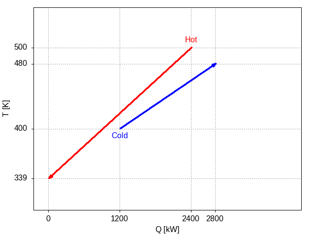
Figure 1: Plot of a hot stream and a cold stream showing the potential for heat exchange between the two streams.
where the overlap between the projections of the hot and cold streams onto the x-axis is a measure of the potential heat that can be exchanged between the two streams.
In this post, I would like to demonstrate the potential of this graphical approach for an optimization based design procedure.
An example problem
A typical benchmark problem consists of 5 hot streams and 5 cold streams (Lewin 1998). Details in the following in table 1.
| Label | Tin | Tout | Q |
|---|---|---|---|
| [K] | [K] | [kW] | |
| H1 | 433 | 366 | 589 |
| H2 | 522 | 411 | 1171 |
| H3 | 544 | 422 | 1532 |
| H4 | 500 | 339 | 2378 |
| H5 | 472 | 339 | 2358 |
| C1 | 355 | 450 | 1642 |
| C2 | 366 | 478 | 1557 |
| C3 | 311 | 494 | 1545 |
| C4 | 333 | 433 | 762 |
| C5 | 389 | 495 | 645 |
| Steam | 509 | 509 | |
| Water | 311 | 355 |
An algorithm for graphical layout of line segments
In the previous post, we showed how we could draw hot and cold streams in a 2d temperature versus heat plot. The key insight is that an exchange of heat from a hot stream to a cold stream is possible if these two streams overlap in their projection onto the x axis and if the hot stream lies above the cold stream throughout the interval defined by their intersection in the projection. The task is to draw these streams in such a way as to maximise the amount of exchange.1
With the example in the previous post, the optimization problem would be one of considering different positions for the single cold stream when placed below the hot stream. When there are more streams, the problem is combinatorial. My solution to this problem is to define a greedy (but not excessively so) algorithm where some simple heuristics will enable the identification of hopefully good solutions.
A layout will be defined by the order in which we consider placing the streams in the graphical presentation. Given an order (a permutation list of indices, from 1 to the total number of streams), the algorithm is
for each stream s in given order
    x ← max(end point of previous stream of same type,
            position that maximises exchange with previous stream
              of opposite type)
    place line @ x
    if line placement infeasible
       shift line to the right to make match feasible
    end
end
This is a greedy algorithm in that it does not consider all possible options in the placement of an individual stream. However, if all different orderings of the streams would be considered (which would potentially take a very long time, O(n!) for n being the number of streams), the search space will include good solutions although possibly not the actual global optimum.2 There is always a trade-off between the size of a search space for optimization and the computational work required to search the space effectively. The greedy approach here should identify good solutions hopefully quickly.
Actual code (with all comments removed to minimise space):
function place(layout)
    ns = length(layout.streams)
    zeroQ = 0.0*unit(layout.streams[1].Q)
    streams = [layout.streams[layout.order[i]] for i in 1:ns]
    lines = Line[]
    lastcold = nothing
    lasthot = nothing
    for i ∈ 1:ns
        s = streams[i]
        if ishot(s)
            x = max( lasthot == nothing ? zeroQ : lasthot.p2.x,
                     lastcold == nothing ? zeroQ : lastcold.p2.x-s.Q,
                     lastcold == nothing ? zeroQ : lastcold.p1.x )
            hotline = Line(s, x)
            if lastcold != nothing && ! isFeasible(hotline, lastcold, layout.problem.ΔTmin)
                hotline = Line(s, lastcold.p2.x)
            end
            push!(lines, hotline)
            lasthot = hotline
        else
            x = max(lasthot == nothing ? zeroQ : (lasthot.p2.x - s.Q),
                    lasthot == nothing ? zeroQ : lasthot.p1.x,
                    lastcold == nothing ? zeroQ : lastcold.p2.x)
            coldline = Line(s, x)
            if lasthot != nothing && ! isFeasible(lasthot, coldline, layout.problem.ΔTmin)
                coldline = makeFeasible(lasthot, coldline, layout.problem.ΔTmin)
            end
            push!(lines, coldline)
            lastcold = coldline
        end
    end
    return lines
end
One aside: all quantities in the package, including heat duties and temperatures, have units associated with them. I use the Unitful.jl package to handle units. This is why the third line in the code is necessary:
zeroQ = 0.0*unit(layout.streams[1].Q)
as I need to consider a heat rate of 0 in the following code. This rate has to have the appropriate units so that it can be used in calculations involving heat rates.3
To illustrate what this algorithm does, consider the problem table defined above. There are 10 streams for on the order of 3 million possible orderings. One order would be as listed in the table. The result of the algorithm above for this ordering is
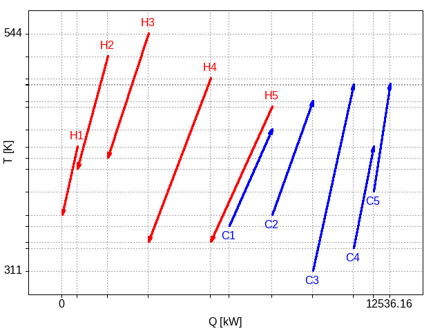
Figure 2: Plot of the hot and cold streams based on an ordering of all the hot streams followed by all the cold streams.
The hot streams are placed first. The first cold stream can be placed so that it lies partly below the last hot stream. The remaining cold streams are placed contiguously after that first one. This is not necessarily a good design: there is only exchange of heat between streams H5 and C1.
If we, instead, consider an order which interleaves the hot and cold streams, the resulting layout is
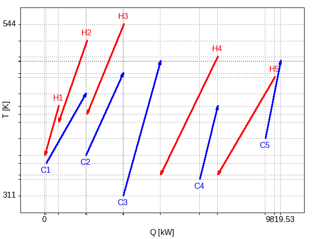
Figure 3: Plot of the hot and cold streams based on an ordering where the hot and cold streams are interleaved.
Here we see that each cold stream has been given the opportunity to be involved in a heat exchange with one of the hot streams. Further, one of the hot streams, H2, has also been placed to match with a cold stream. Stream C3 is not integrated with any hot stream, however.
The overall outcome is a potentially much better design as a significant amount of heat can be exchanged. But it's not necessarily the best we can do. To do better, we have to search the space of alternative orderings of the streams: an optimization problem.
Design of network using a nature inspired optimization method
The optimization method I use is Fresa, an evolutionary method, inspired by plant propagation, specifically one of the methods strawberries use to propagate. Fresa, out of the box so to speak, supports problems where the decision variables are real and/or integer variables in a bounded domain with or without equation based constraints. The decision variables for the heat exchanger network design problem, however, are represented by a permutation of the first n integer numbers.
To apply Fresa to such a problem, we need to define a neighbour function, a function that generates new points in the search space from a given point. For this problem, the neighbour function I have defined is
function Fresa.neighbour(l :: Layout, ϕ, domain)
    order = copy(l.order)
    nswaps = ceil(Int,(1-ϕ)*5)
    for i in 1:nswaps
        indices = rand(1:length(order), 2)
        order[reverse(indices)] = order[indices]
    end
    Layout(order, l.streams, l.problem)
end
where order is a permutation vector of the first n positive integer numbers and ϕ ∈ (0,1) is the fitness of the solution (i.e. the layout) passed to this function. The most fit solutions in a population will have fitness values close to 1; the least fit will have values closer to 0.
The function above takes a given permutation order and performs a number of swaps of 2 of the integer values in the permutation, the number of swaps being inversely related to the fitness. The most fit solutions will typically identify neighbouring solutions with only one swap; the least fit will identify neighbours with up to 5 swaps.
Using this neighbour function, we can now try to solve the heat exchanger network design problem. The best layout found, typically in less than 100 generations and around 1000 different layouts considered (around 7 seconds elapsed time), is
![Plot of the optimum placement found by Fresa for the problem defined in Table [[lewinCtable]].](images/qthen-lewin-c-best-layout.png)
Figure 4: Plot of the optimum placement found by Fresa for the problem defined in Table 1.
The order in which the streams are placed is
[2, 10, 8, 3, 5, 6, 4, 7, 1, 9]
which corresponds to streams
[H2, C5, C3, H3, H5, C1, H4, C2, H1, C4]
From this graphical representation, we see that the network identified meets almost all of the heating requirements for the cold streams, all but a small bit of heating for C4. Cooling with external utilities is required for all the hot streams except for H3.
In the next post, I will discuss cases where this greedy approach is unable to find potentially better solutions, including the example presented here where better solutions are definitely possible yet cannot be represented with the current placement algorithm described above.
Blog navigation
| Previous post | Blog | Next post |
|---|---|---|
| QTHEN: 1. Inspiration from visualization for heat exchanger network design | Index | Emacs carnival: Elevator pitch (or How I learned to love RSS for the fediverse) |
You can find me on Mastodon or you can email me should you wish to comment on this entry or the whole blog.
References
Footnotes:
Actually, we typically will want to minimise an economic criterion. This will typically be the annualised cost of the heat exchange network. The annualised the cost includes capital costs, for building and installing the heat exchangers, and operating costs, based on the consumption of external utilities. In the table, the utilities available are included although not their costs. Refer to the paper cited above for all the costing details.
The next post in this series on heat exchanger network design, when I get around to writing it, will consider a larger more complex search space, one which should be able to identify optimal solutions (maybe). But the intention is to use this greedy algorithm as the basis for a two level optimization approach.
As a computer scientist working in process systems engineering, it dismays me that very few software packages handle units of measure properly if at all. Few modelling systems allow the use of units and, even when they do, they often cannot handle automatic conversion of units where required. There are exceptions to this, of course. Being able to handle units for all quantities that should have these makes for better software as many errors can be caught when calculations have incompatible units, for instance.