QTHEN: 3. Motivating stream splitting and cutting for heat exchanger network design
A previous blog post showed that a greedy algorithm for stream placement in a two-dimensional Q and T diagram was able to identify good heat exchanger network designs. However, this algorithm fails in some cases to identify good designs. In this post, I illustrate two such cases and use these to motivate a two level optimization approach.
Case 1: stream cutting
Consider the following problem table, a subset of the problem table presented in the previous blog mentioned above:
| Label | Tin | Tout | Q |
|---|---|---|---|
| [K] | [K] | [kW] | |
| H1 | 433 | 366 | 589 |
| H2 | 522 | 411 | 1171 |
| C1 | 311 | 494 | 1545 |
| Steam | 509 | 509 | |
| Water | 311 | 355 |
The optimum layout (as identified by the greedy layout algorithm) is shown here:
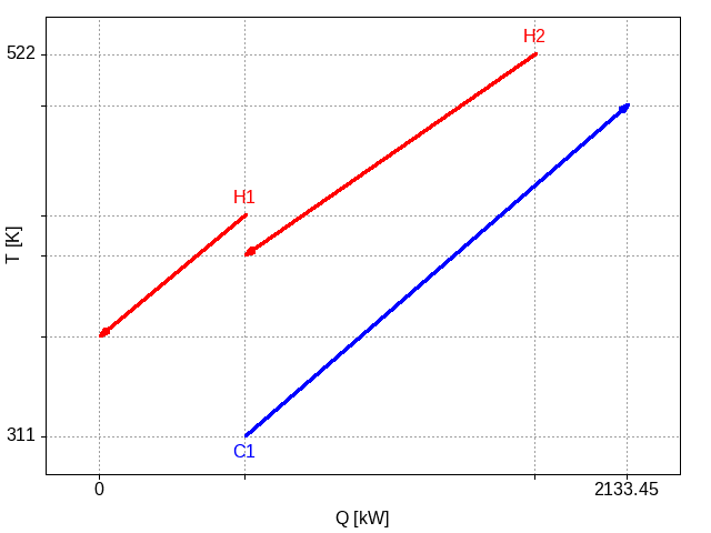
Figure 1: Plot of the two hot streams and the single cold stream, showing heat transfer between the second hot stream and the single cold stream.
The integration identified meets all the cooling requirements of the H2 hot stream which is a good outcome. However, a better design is immediately apparent: we could shift the cold stream to the left, still meeting all the requirements of H2 but also then meeting some of the requirements of H1. The algorithm described in the previous post cannot achieve such a solution:
- if the hot streams are placed first, the cold stream can only be placed to match with the second hot stream. This is due to the greedy nature of the algorithm, avoiding a full combinatorial and tunable search of all positions of the stream;
- if the cold stream is placed before the second hot stream, the second hot stream cannot be placed to integrate with the cold stream as it would violate the driving force requirement of a minimum temperature difference.
A solution, based on the graphical representation, is to consider a modified problem table where we cut the cold stream into two segments:
| Label | Tin | Tout | Q |
|---|---|---|---|
| [K] | [K] | [kW] | |
| H1 | 433 | 366 | 589 |
| H2 | 522 | 411 | 1171 |
| C1a | 311 | 355.3 | 374 |
| C1b | 355.3 | 494 | 1171 |
| Steam | 509 | 509 | |
| Water | 311 | 355 |
This cutting of the stream does not change the underlying problem. It is simply representing the cold stream using two contiguous segments. However, it enables the layout algorithm to place each segment separately and the following layout is possible:
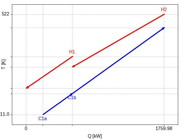
Figure 2: Plot of the two hot streams and the two segments of the cold stream, showing heat transfer now between both hot streams with the cold stream.
This new configuration leads to a reduction in capital cost of around 4% and, more significantly, a reduction in utility costs of 93%.
Cutting stream C1 into two segments, as was done in generation problem table 2 from table 1, means that the stream first flows through an exchanger (obtaining heat from H1) and then flows through a second exchanger (with H2).
Case 2: stream splitting
An alternative to cutting a stream into segments is to consider splitting the flow of a given stream into multiple separate streams. I illustrate this with the following example problem table (subset of case study A from (Lewin 1998)):
| Label | Tin | Tout | Q |
|---|---|---|---|
| [K] | [K] | [kW] | |
| H2 | 480 | 360 | 480 |
| H3 | 460 | 360 | 600 |
| C1 | 340 | 460 | 1200 |
| Steam | 700 | 700 | |
| Water | 300 | 320 |
The best layout found for this small problem is
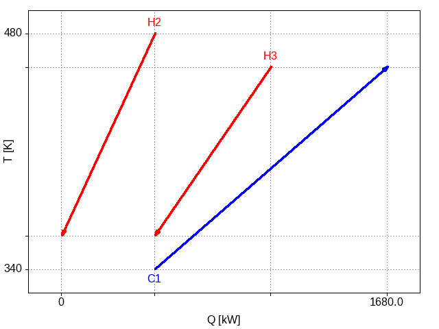
Figure 3: Plot of the two hot streams and the single cold stream for the second example.
In this case, it is not immediately apparent how to do better. However, the slope of each line indicates how much the temperature will change for a unit of heat. The cold stream has a smaller change in temperature for each kilowatt of energy it receives; the hot streams have greater changes in temperature for each kilowatt of heat taken away. The slopes of the lines give a visual indication that splitting the cold stream into two streams with higher slopes may lead to a greater potential for exchange. For instance, consider this modified problem table:
| Label | Tin | Tout | Q |
|---|---|---|---|
| [K] | [K] | [kW] | |
| H2 | 480 | 360 | 480 |
| H3 | 460 | 360 | 600 |
| C1a | 340 | 460 | 480 |
| C1b | 340 | 460 | 720 |
| Steam | 700 | 700 | |
| Water | 300 | 320 |
The cold stream has been split into two streams, each with the same inlet and outlet temperatures but with different amounts of heat required (amounts adding up to the total amount for C1 in Table 3). One possible integration layout for this problem is
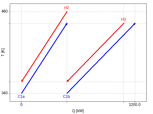
Figure 4: Plot of the two hot streams and two cold streams that arise from splitting the original single cold stream.
The result is that all of the cooling requirements for both hot streams are met by process integration. Only a little amount of heating using utilities is required for the cold stream.
This solution, interestingly, has a higher capital cost, approximately 40% higher, due to the smaller driving forces for the integrated exchanges. However, the utility requirements have dropped by approximately 81%. Depending on the economic conditions (primarily the costs of external energy sources), the solution in Figure 4 may be a better solution or it may be that Figure 3 is better. Note that the new design likely better from an environmental perspective. In any case, being able to consider cases with stream splitting gives the designer more options.
Optimization with cutting and splitting options
The possibility of cutting and splitting streams should be considered in an optimization procedure for heat exchanger network when the greedy algorithm for stream placement graphically forms the basis of the design. I will discuss how to do this in a following post (soon hopefully).
Blog navigation
| Previous post | Blog | Next post |
|---|---|---|
| Emacs carnival: Elevator pitch (or How I learned to love RSS for the fediverse) | Index | QTHEN: 4. A representation for heat exchanger network configurations |
You can find me on Mastodon or you can email me should you wish to comment on this entry or the whole blog.