QTHEN: 1. Inspiration from visualization for heat exchanger network design
The heat exchanger network design problem
One very interesting (and challenging) problem in the design of chemical process plants is how to make use of excess heat in one part of a process to meet heating requirements in other parts of the process. The solution to this problem is a heat exchanger network. A network consists of hot streams, streams which need to be cooled, and cold streams, those which need to be heated. In the network, heat exchangers are placed to enable the transfer of heat from hot steams to cold streams. A review of the design of heat exchanger networks can be found in Chapter 3 of (Towler and Sinnott 2013).
Identifying the best such network is a challenging optimization problem. This problem has been the focus of research in optimization methods and modelling for a long time (Fraga, Patel, and Rowe 2001; Zamora and Grossmann 1998; Morton 2002; Floudas, Ciric, and Grossmann 1986; Linnhoff and Hindmarsh 1983; Linhoff and Flower 1978). The problem is typically formulated as a mixed integer nonlinear programme (MINLP) representing a superstructure of all the possible structures or networks.
The first paper cited above (Fraga, Patel, and Rowe 2001) is interesting, not because it is one of my own 😉, but because it uses a visual representation of solutions to the problem as the basis for optimization. The basic concept is described here as it will form the basis for a new Julia package for heat exchanger network design, working title QTHEN. The intention is to address some of the short-comings of the approach taken in that paper.
Small example problem
The following table, known as a problem table, presents two streams, one hot and one cold:
| Stream | Inlet | Outlet | Heat |
|---|---|---|---|
| [K] | [K] | [kW] | |
| Hot | 500 | 339 | 2400 |
| Cold | 400 | 480 | 1600 |
The hot stream needs to be cooled from 500 K to 339 K by giving away 2400 kW of heat in doing so. The cold stream needs to receive 1600 kW of heat to increase its temperature from 400 K to 480 K.
Visualization
We can display this information graphically, in this case using gnuplot (more on how we use gnuplot below), showing the above streams with temperature, T, versus rate of heat to transfer, Q:
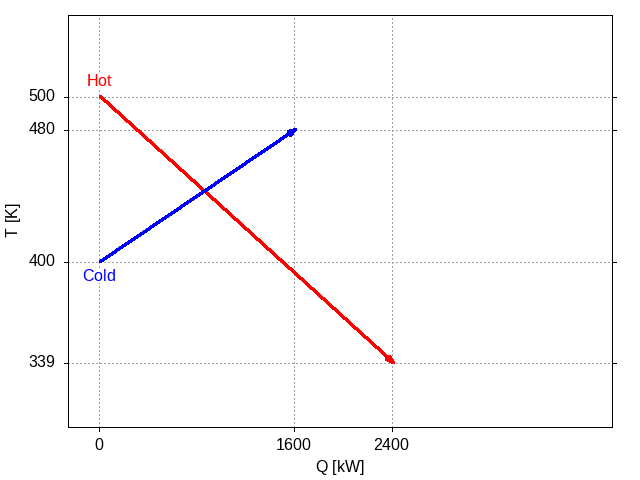
Figure 1: Plot of two streams, each defined by their inlet and outlet temperatures and the rate of heat.
In this plot, the hot stream is represented by a line showing that this stream needs to be cooled from 500 K to 339 K, shedding heat at a rate of 2400 kW. The cold stream is drawn to show that it needs to be heated from 400 K to 480 K, with a rate of heat to be added to the stream of 1600 kW. The vertical and horizontal dotted lines help visualise the start and end of each stream in this problem.
We call this type of diagram a QT diagram.
The intersection of the two lines is of interest. We can use Emacs Calc to find this intersection, using the symbolic algebra capabilities of Calc directly in our text buffer in Emacs. The equations representing the two lines are:
[calc-defaults]
[calc-mode: float-format: (eng 4)]

hot := T = ((339 - 500) / 2400) Q + 500 => T = 500 - 67.08e-3 Q

cold := T = ((480 - 400) / 1600) Q + 400 => T = 50e-3 Q + 400
where we have included some directives for embedded calc mode, resetting to defaults and specifying engineering notation for numbers.
The intersection point is where the two lines have the same values of T and Q:
solve([hot, cold], [T, Q]) => [T = 442.7e0, Q = 854.1e0]
The basis for heat exchange from one stream to another is the concept of a temperature driving force (second law of thermodynamics). This means that heat can transfer from a stream at a higher temperature to one at a lower temperature. This plot illustrates that there is some potential to transfer heat from the highest temperature range of the hot stream to the coldest range of the cold stream. The absolute limit (and one which cannot be reached) is the point of intersection. This tells us that we could exchange up to some amount less than Q = 854 kW of heat between the two streams.
The example illustrated above involves co-current heat exchange, where both streams come into a heat exchanger from the same end and both exit at the other end, exchanging heat while flowing through the heat exchanger. In practice, however, many heat exchangers are designed for counter-current operation where the two streams enter at opposite ends of the exchanger and flow in opposite directions.
We are going to consider some alternative configurations for the streams, displaying each configuration using gnuplot. All alternatives will use the same code, using the CALL org mode keyword for calling src blocks. The src block in this case is
reset
# show box around plot
set border 15
# tic marks only on main axes
set xtics nomirror
set ytics nomirror
# do not show a key for the plot
unset key
# get rid of ugly box around text labels
set style textbox 2 opaque noborder
# have the tic marks extend as grid lines through the plot
set grid xtics
set grid ytics
# label the hot and cold streams
set label 'Hot' at Qh,Thin center offset 0,1 textcolor 'red' boxed bs 2
set label 'Cold' at shift,Tcin center offset 0,-1 textcolor 'blue' boxed bs 2
# draw the two streams
set arrow from Qh,Thin to 0,Thout lc 'red' lw 3.0
set arrow from shift,Tcin to (Qc+shift),Tcout lc 'blue' lw 3.0
# label and define the x axis
set xlabel 'Q [kW]'
set xrange [-250:4250]
# convert from org variables to entities suitable for use by the xtics
# command
Qcstart = sprintf("%s", shift)
Qcend = sprintf("%d", Qc+shift)
# set the tic marks to match the start and end of each the two streams
set xtics ( "0" 0.0, Qh Qh, Qcstart Qcstart, Qcend Qcend ) nomirror out
# similar for the y axis
set ylabel 'T [K]'
set yrange [300:550]
set ytics ( Tcin Tcin, Tcout Tcout, Thin Thin, Thout Thout ) out
# gnuplot will not generate anything unless we actually ask it to plot
# something.  Here we plot a point at the origin which is not within
# the domain or range of the graphics drawn so will be hidden.  Kind
# of sneaky... ;-)
plot '< echo 0 0'
This script, named qthen-twostream-example-draw-countercurrent-with-shift, will generate a plot where the values for the hot and cold stream temperatures and heat duties have been defined for use by gnuplot using the following header variables:
#+header: :var Thin=hensimpleproblemtable[3,1]
#+header: :var Thout=hensimpleproblemtable[3,2]
#+header: :var Qh=hensimpleproblemtable[3,3]
#+header: :var Tcin=hensimpleproblemtable[4,1]
#+header: :var Tcout=hensimpleproblemtable[4,2]
#+header: :var Qc=hensimpleproblemtable[4,3]
These header variables make reference to the simple problem table given above, named hensimpleproblemtable. If we were to update the table with different temperatures and heat requirements, the plots would update automatically.
A variable, shift, is also used to shift the cold stream to the right. We will invoke the above script using the CALL keyword as:
#+CALL: qthen-twostream-example-draw-countercurrent-with-shift[:eval yes :var shift=0 :file images/qthen-twostream-example-countercurrent.png]()
where we provide a value of the shift variable and the desired destination for the generated plot (the :file specification).
With no shift at all, :var shift=0, the graphical representation is:
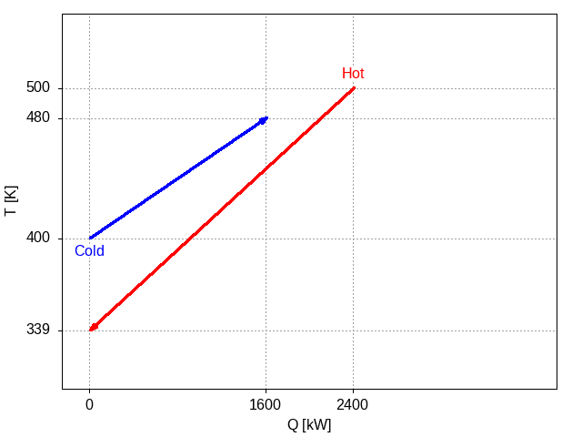
Figure 2: Plot of two streams, each defined by their inlet and outlet temperatures and the rate of heat, with cold flowing from left to right and hot flowing in the opposite direction, from right to left.
In this plot, the hot stream is represented by a right to left line showing that this stream needs to be cooled from 500 K to 339 K, shedding heat at a rate of 2400 kW. The cold stream is drawn left to right and it needs to be heated from 400 K to 480 K, with a rate of heat to be added to the stream of 1600 kW.
When drawn this way, there is no point where the hot stream lies above (higher temperature) than the cold stream. This seems to indicate that there is no scope for heat exchange from the hot stream to the cold stream using a counter-current heat exchanger.
However, although the temperatures of the streams are absolute quantities, the rate of heat for each stream is the required change in the heat of each stream. Therefore, we can place these streams anywhere along the x axis. It is the width of the projection of each stream onto the x axis that represents the rate of heat required. For example, we could draw the two streams in this way, shifting the cold stream to the right by 2400 kW:
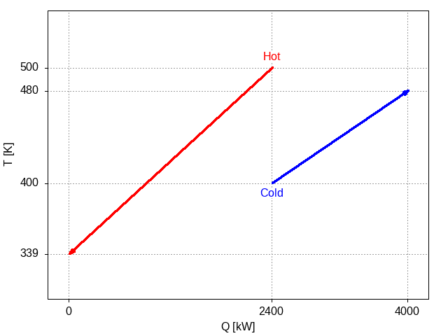
Figure 3: Plot of the two streams with the cold stream shifted to the right by 2400 kW.
This is not very interesting as there is no place where the hot stream lies above the cold stream. In other words, no heat exchange is indicated in this configuration. However, we can see visually that exchange would be possible were we to slide the cold stream under the hot stream by shifting it to the left. The next plot shows the configuration resulting from shifting the cold stream only 1200 kW from the origin instead of 2400 kW:
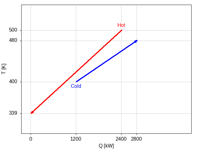
Figure 4: Plot of the two streams with the cold stream shifted to the right by 1200 kW.
In this view, we can see that the hot stream lies above the cold stream throughout the domain where these two streams overlap (in a projection onto the x axis). There are three regions, defined by the vertical dotted lines. The first region from the left, (0,1200) kW, represents the part of the hot stream that needs cooling from external sources. The second region, (1200, 2400) kW, is where the hot stream can shed heat to be accepted by the cold stream; this is known as heat integration or process integration. The third and final region, (2400,2800) kW, represents the part of the cold stream that must receive heat from some external source.
In this case, the rate of heat integrated is 1200 kW, significantly more than could be achieved with co-current exchange (see Figure 1). This is attractive when minimising external energy use (heating and cooling utilities).1
This graphical view of what heat exchange is possible motivates an optimization procedure to identify the best heat exchanger network when given a set of hot and cold streams and external utilities to make up any heating or cooling that cannot be achieved through exchange of heat between streams in the process. For instance, the horizontal position of lines representing both hot and cold streams, the shift, could be the decision variable for optimization. In the paper discussed above (Fraga, Patel, and Rowe 2001), the horizontal position was based on an actual graphical display. In that case, the decision variable was an integer so the problem was one of discrete optimization. In QTHEN, we will consider a generalisation of this where the position can be specified by a real number.
The problem is one with infeasible solutions. An example of such is shown here:
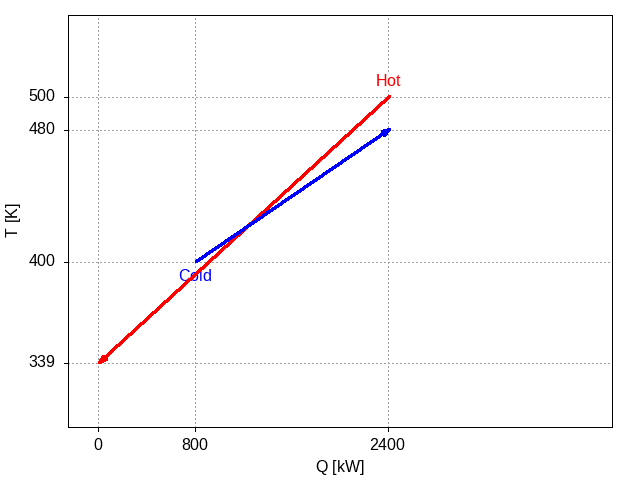
Figure 5: Plot of the two streams where the shift of 800 kW results in the two streams intersecting
In this example, we have tried to shift the cold stream to attempt to meet all of its heating requirements from the hot stream. However, we see that for part of the domain, the cold stream lies above the hot stream, violating the second law of thermodynamics.
Following posts will present the code as it is developed, in the form of a Julia package called QTHEN.
Blog navigation
| Previous post | Blog | Next post |
|---|---|---|
| Emacs carnival: Writing experience | Index | QTHEN: 2. A greedy (but not excessively so) algorithm for optimising stream placement |
You can find me on Mastodon or you can email me should you wish to comment on this entry or the whole blog.
References
Footnotes:
The economics are more complicated however as they depend on the driving forces, the cost of construction, and the cost of the utilities, resulting in a complex typically nonlinear objective function for optimization. More on this to follow in subsequent posts.