1.01 Winding numbers and the fundamental theorem of algebra

(1.45) Let \(p\colon\mathbf{C}\to\mathbf{C}\), \(p(z)=z^n+a_{n-1}z^{n-1}+\cdots+a_0\), be a complex polynomial. Assume that \(p\) has no complex root, in other words that there is no point \(x\in\mathbf{C}\) for which \(p(x)=0\). We will show that \(n=0\), in other words that \(p\) has only a constant term.

(2.24) Consider the circle of radius \(R\) in the complex plane. The points in this circle are precisely those of the form \(Re^{i\theta}\). Let \(\gamma_R\) be the image of this circle under the map \(p\colon\mathbf{C}\to\mathbf{C}\). We can think of \(\gamma_R\) as a loop in \(\mathbf{C}\): \[\gamma_R(\theta)=p(Re^{i\theta}).\] Crucially, because \(p(z)\neq 0\) for all \(z\in\mathbf{C}\), the loop \(\gamma_R\) is a loop in \(\mathbf{C}\setminus\{0\}\).

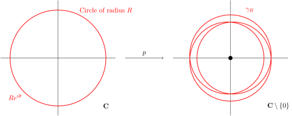
Figure 1. In this figure, we see the circle of radius \(R\) in the domain of \(p\) and its image \(\gamma_R\) in the image of \(p\) (\(\mathbf{C}\setminus\{0\}\)). In this example, \(p(z)=z^3-z/2\) and \(R=2\) and we see that the winding number of \(\gamma_R\) is 3.

(3.54) When \(R=0\), \(\gamma_0(\theta)=p(0)\) is independent of \(\theta\). In other words, \(\gamma_0\) is the constant loop at the point \(p(0)\in\mathbf{C}\setminus\{0\}\).

(4.42) When \(R\) is very large, the term \(z^n\) dominates in \(p\), so \(\gamma_R(\theta)\approx \delta(\theta)\), where \(\delta(\theta)=R^ne^{in\theta}\).

Claim: (6.54) There is a homotopy invariant notion of winding number around the origin for paths in \(\mathbf{C}\setminus\{0\}\) which gives zero for the constant loop and \(n\) for the loop \(\delta(\theta)=R^ne^{in\theta}\).

Homotopy invariant means, roughly, invariant under continuous deformations; in our situation, that means that the winding number of \(\gamma_R\) around the origin should be independent of \(R\). Since \(\gamma_0\) has winding number zero and \(\gamma_R\) has winding number \(n\) for large \(R\), this implies \(n=0\).