1.02 Paths, loops, and homotopies
Video
Below the video you will find accompanying notes and some pre-class questions.
- Previous video: 1.01 Winding numbers and the fundamental theorem of algebra.
- Next video: 1.03 Concatenation and the fundamental group.
- Index of all lectures.
Notes
(0.00) In this section, we're going to introduce the idea of continuous paths, loops and homotopies of loops. I will assume you're happy with the notions of topological space and continuous maps between topological spaces. If you haven't come across these ideas, I have a series of videos covering these ideas which you can watch at any point during the module. If you like, you can mentally replace the word ``topological space'' with ``metric space'' until you've watched those videos.
Paths
(1.06) Let \(X\) be a topological space. A path in \(X\) is a continuous map \(\gamma\colon[0,1]\to X\). You can think of this as a continuous parametric curve \(\gamma(t)\) with parameter \(t\in[0,1]\).
The map \(\gamma(t)=(t,0)\) is a path in the plane \(X=\mathbf{R}^2\) which moves along the \(x\)-axis from \((0,0)\) to \((1,0)\).
The map \(\gamma(t)=(\cos(2\pi t),\sin(2\pi t))\) is another path in the plane which moves around the unit circle. This is a loop (it starts and ends at the same point \((1,0)\).
A path \(\gamma\colon[0,1]\to X\) is called a loop if \(\gamma(0)=\gamma(1)\). It is said to be a loop based at \(x\) if \(\gamma(0)=\gamma(1)=x\).
Free homotopy of loops
(4.06) Roughly speaking, a free homotopy of loops is a continuous one-parameter family of loops \(\gamma_s(t)\) interpolating between two loops \(\gamma_0(t)\) and \(\gamma_1(t)\). More precisely:
A free homotopy of loops is a continuous map \(H\colon [0,1]\times[0,1]\to X\) such that \(\gamma_s(t):=H(s,t)\) is a loop for each fixed \(s\in[0,1]\), that is \(H(s,0)=H(s,1)\) for all \(s\in[0,1]\).
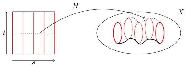
Figure 1. In this figure, we see the domain and target of a free homotopy \(H\colon[0,1]\times[0,1]\to X\). The loops \(\gamma_s(t)=H(s,t)\) are indicated in red for \(s=0,\frac{1}{4},\frac{1}{2},\frac{3}{4},1\). The path traced by basepoints is drawn in thick black; as a visual aid, the path traced by the midpoints of the loops is also drawn in dotted black.
We will often write \(\gamma_s\) instead of \(H\) to emphasise the fact that \(H\) is a family of loops.
Continuity of \(H\) as a map of two variables is what gives us a continuous family of continuous loops.
Based homotopy of loops
(7.53) We will need a slightly more restricted notion of homotopy.
If \(x\in X\) is a basepoint, a homotopy based at \(x\) is a homotopy \(H\colon[0,1]\times[0,1]\to X\) where \(H(s,0)=H(s,1)=x\) for all \(s\in [0,1]\). In other words, all the loops \(\gamma_s(t)=H(s,t)\) pass through the basepoint \(x\) at \(t=0,1\). If we have a based homotopy \(\gamma_s\) we will write \(\gamma_0\simeq\gamma_1\) and say that \(\gamma_0\) is homotopic to \(\gamma_1\).
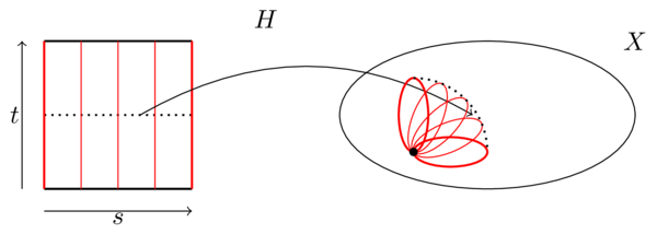
Figure 2. A picture of a typical based homotopy. The basepoint is the black dot on the right; both top and bottom edges of the domain map to the basepoint.
By focusing on based loops (and based homotopy) we will be able to concatenate loops (because they all start and end at the same point) and this will give us a group structure on (homotopy classes of) loops.
Loops in \(\mathbf{R}^n\) are contractible
(11.04) If \(\gamma\colon[0,1]\to\mathbf{R}^n\) is a loop based at the origin \(0\) then \(\gamma\) is based-homotopic to the constant loop \(t\mapsto 0\).
The map \(H(s,t)=(1-s)\gamma(t)\) is a continuous map such that \(H(s,0)=0=H(s,1)\), so it is a based homotopy. At \(s=0\), we get \(\gamma_0(t)=H(0,t)=\gamma(t)\). At \(s=1\), we get \(\gamma_1(t)=H(1,t)=0\), so this is a based homotopy from \(\gamma\) to the constant loop.
A homotopy from a loop \(\gamma\) to a constant loop is called a nullhomotopy (and we say that \(\gamma\) is contractible if it is nullhomotopic).
Pre-class questions
- Is the homotopy \(\gamma_R\) from the previous video a based homotopy or a free homotopy?
Navigation
- Previous video: 1.01 Winding numbers and the fundamental theorem of algebra.
- Next video: 1.03 Concatenation and the fundamental group.
- Index of all lectures.