This is the pdf file of my project (if you prefer doubled sided please use this link). All of the zip files on here are password protected. If you wish to open this the password is contained in project you recieved, alternatively you may contact me using the e-mail address on my home page requesting a password. The pictures an animations below are free for you to view without needing a password. If you wish to see more of what went behind it and all the pretty pictures and animations compiled during the theoretical side of it please keep on reading below.
These were experiments conducted at NIOZ, there is a matlab file with each batch of experiments and the data files and photos are available in a zip file here (approximately 70MB) and the analysis of a few select examples is available at the start of the main project pdf or alternatively, the analysis of all the experiments conducted is available here.
With each of the more recent experiments the initialisation (.ini) file is included with the data, giving an outline of which setting were used. In the initialisation file the top and bottom row correspond to the table and pump voltage respectively.
Below are links to the most important pictures and animations, Here is a link to a zip file of all of them, including the matlab and mathematica files used to generate them (approximately 95MB). All .mat files are matrices of co-efficients to be imported into Mathematica if you choose to compute plots. Further descriptions are given on this page.
.jpg and .png files are plots and .gif file are animations. The mathematica files are slightly rough and not very well presented as the functions are very well presented in the built in help functions, but the matlab files are quite neat with explanations as you go along.
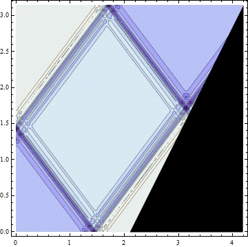
If you have the full pack then the three numbers x-y-z are the number of points taken in the first fundamental interval, second fundamental interval and lower half of the slope respectively. Clipped was a method I used to reduce the condition number of the matrix of co-efficients which needed to be inverted. Some are contour plots others are density plots (which I found to be inferior and desisted from computing) which will be obvious from the title, if neither are mentioned it is a contour plot.
In some of these I haven't drawn the wall in at the right hand side, you'll have to imagine it. It goes from the top right hand corner, through the corner of the attractor down to y=2pi/3, z=0.
If you have the full pack some begin with 3D which means it is a 3D animation, the others are a contour plots. All will contain at some point an isolated letter u, v or p which means the plotted value is that of u, v or p. Occasionally this will be writen in the form "contouru", "contourv" or "contourp" which is the name I used in Mathematica. The value of k is clearly specified as "k=..."with k real implying propagating, k imaginary implying decaying and k complex a mixture of the two. Omega is usually specified, despite almost always being one half.
In some of these I haven't drawn the wall in at the right hand side, you'll have to imagine it. It goes from the top right hand corner, through the corner of the attractor down to y=2pi/3, z=0.
_flat_box_intersecting_animation.gif)
_flat_box_intersecting_animation.gif)
_flat_box_intersecting_animation.gif)