E S Fraga: Jacaranda blog
Table of Contents
Introduction
This document presents a collection of notes and news items for the Jacaranda system for automated design and optimisation sorted in reverse chronological order.
Visit my home pages for links to my pages on general research, teaching and other interests.
Direct flowsheet definition
Although Jacaranda was explicitly created for the automated design of processes, including heat exchanger networks, there are times when one may wish to investigate the behaviour of a particular given process. Jacaranda provides a Flowsheet class for just this purpose. An instance of this class can be defined directly by the engineer or as the result of an automated design run in Jacaranda. This blog entry will focus on the user defined case.
A flowsheet consists of a set of units and their connections. Connections are represented by streams. To define a flowsheet, we first define the units and the streams and finally tell Jacaranda how they come together.
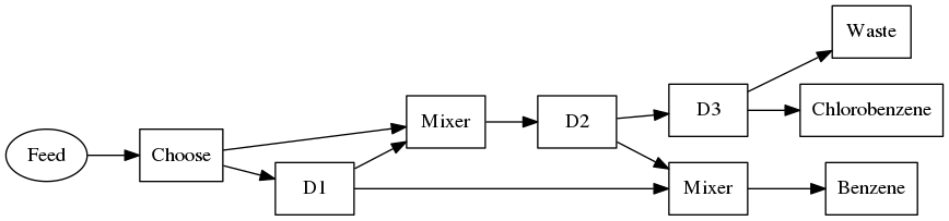
The following is an example of a superstructure flowsheet. A superstructure is a representation of multiple structures and is the basis for alternative automated design procedures, often through the use of generic MINLP solvers such as those available through GAMS. Jacaranda also has a range of MINLP solvers, mostly based on stochastic optimisation methods but also direct search methods.
The superstructure consists of three distillation units. A valid process in this example could consist of just two distillation units but a three distillation unit process is actually less expensive to operate under specific conditions. It is worth exploring the trade-offs between the two options through the use of a single superstructure Flowsheet object.
We consider the separation of a mixture which is actually the output of a reaction unit used for the chlorination of benzene. The feed to the separation section is 97% Benzene (component A below), 1% C6H5Cl (B), 1% p-C6H4Cl2 (C), and 1% C6H3Cl3 (D). The aim is produce pure Benzene (>98% purity) and somewhat pure C6H5Cl (>90% purity). The other two components are waste products and come out with any purity. We want less than 1% of any of the waste products in the Benzene output stream. Short cut design methods based on the Fenske-Underwood-Gilliland model.
The rest of this blog entry is a description of the input file for this process. We start with some general settings:
# start by specifying that all objects come from the Jacaranda
# package, specifically the process synthesis sub-package and the unit
# models. We turn on assertions to catch any silly errors as we are
# still debugging some of this code

use jacaranda.design.ps
use jacaranda.design.units

# define some global variables

variables
 # the discretization of component flows
 const Base 0.001 "Base component flow discretization"
 # define the flows of the components in the feed
 const Fbenzene  0.97 "Flow of Benzene in feed stream"
 const Fc6h5cl   0.01 "Flow of C6H5Cl in feed stream"
 const Fpc6h4cl2 0.01 "Flow of p-C6H4Cl2 in feed stream"
 const Fc6h3cl3  0.01 "Flow of C6H3Cl3 in feed stream"
 # set the cost base to 1993 based on the M&S index
 set msindex 964.2
 # and the number of discrete enthalpy (or state) levels for streams.
 # it is probably a good idea to have this value match the number of
 # operating pressures in the distillation columns.
 const nPs 4 "Number of discrete stream enthalpy levels"
end

# define the ranking criteria: we want to study the difference in
# operating versus capital costs so we define two criteria, each of
# which is the sum of the relevant criterion value generated by each
# unit in a flowsheet. The term in quotes for each criterion is the
# expression to evaluate for each unit. The "sum" means that the value
# of the criterion is the sum of expression evaluate for all the units
# in the resulting flowsheets.

Criteria costs
 criterion CapitalCost sum "capcost"
 criterion OperatingCost sum "opercost"
end

# define the heat exchanger model for heating and cooling. We define
# two cost functions, one for the capital cost as a function of the
# area of the exchanger, and the other the operating cost as a
# function of the duty (Q [kJ]), the cost of the utility used (Cu
# [$/kJ]), and the time (seconds in a year equal to h*hpy where hpy is
# the "hours per year"). To cater for equal temperature differences at
# both ends of the exchanger, we use the Chen approximation.

HeatExchanger hex
 model
  deltain = abs(T1in-T2out)
   deltaout = abs(T1out-T2in)
  eps = abs(deltain/deltaout-1)
  if eps < 4e-4
     lmtd = (1+eps/2-eps^2/12)*deltaout
  else
     lmtd = (deltain - deltaout)/log(deltain/deltaout)
  endif
  A = Q/U/lmtd
  capcost = 101964 + 92.9*A^0.65
  opercost = Cu*Q*h*hpy
 end
end

# define the utilities available for meeting heating and cooling
# demands from the units. the parameters for each unit are inlet
# temperature, outlet temperature, heat transfer coefficient, and
# cost.

DiscreteUtilities utils
    hot  "Steam @ 28.23 atm"	503.5 503.5   "5000 *W/m^2/K" "1.0246 / GJ"
    hot  "Steam@11.22atm"	457.6 457.6   "5000 *W/m^2/K" "0.773824 / GJ"
    hot  "Steam@4.08atm"	417.0 417.0   "5000 *W/m^2/K" "0.573203 / GJ"
    hot  "Steam@1.70atm"	388.2 388.2   "5000 *W/m^2/K" "0.41796 / GJ"
    cold  "ColdWater@32.2degC"  305.2 305.2   " 500 *W/m^2/K" "0.0668737 / GJ"
    cold  "Ammonia@1degC"	274.00 274.00 " 500 *W/m^2/K" "1.65035 / GJ"
    cold  "Ammonia@-17.68degC" 	255.32 255.32 " 500 *W/m^2/K" "2.96871 / GJ"
    cold  "Ammonia@-21.67degC"	251.33 251.33 " 500 *W/m^2/K" "3.96226 / GJ"
end

# all the data we need for this problem has been defined. Now set the
# global data variables that are used by the synthesis procedure
# before attempting to define the actual synthesis problem.

Data
 criteria costs			# rank according to given criteria
 hex hex			# use heat exchanger model specified
 utils utils
 print				# output all settings
end
With these setting, we can now proceed to define the flowsheet. The first requirement is the definition of the feed stream. This requires us to define the species that appear in the process along with the data required for the estimation of the necessary physical properties, such as bubble and dew points for mixtures.
vle.KistaComponent benzene
 bp 353.2
 cpv -33.917 4.743e-1 -3.017e-4 7.130e-8
 lhtc " 500 *W/m^2/K"
 vhtc "5000 *W/m^2/K"
end

vle.KistaComponent C6H5Cl
 bp 405.2
 cpv -33.888 5.631e-01 -4.521e-04 1.426e-07
 lhtc " 500 *W/m^2/K"
 vhtc "5000 *W/m^2/K"
end

vle.KistaComponent p-C6H4Cl2
 bp 447.3
 cpv  -14.344 5.534e-01 -4.559e-04 1.447e-07
 lhtc " 500 *W/m^2/K"
 vhtc "5000 *W/m^2/K"
end

vle.KistaComponent C6H3Cl3
 bp 486.2
 cpv  -14.361 6.087e-01 -5.622e-04 2.072e-07
 lhtc " 500 *W/m^2/K"
 vhtc "5000 *W/m^2/K"
end
With the components known, we can define the stream as a single liquid phase. The phase composition is defined using the quantities defined earlier. It is also useful to define the base discretisation values although these are not strictly necessary for process simulation and optimisation.
vle.Phase feedPhase
 add benzene Fbenzene
 add C6H5Cl Fc6h5cl
 add p-C6H4Cl2 Fpc6h4cl2
 add C6H3Cl3 Fc6h3cl3

 base benzene	"Base * Fbenzene"
 base C6H5Cl	"Base * Fc6h5cl"
 base p-C6H4Cl2	"Base * Fpc6h4cl2"
 base C6H3Cl3	"Base * Fc6h3cl3"
end
vle.Stream feed
 add feedPhase
 nstates nPs
 T 313
 P "1 *atm"
 print
end
We are now ready to define the units of the process. We start with the feed tank and the product tanks. The latter include the specification constraints that ensure the process designed meets the requirements.
vle.FeedTank feedtank
 Stream feed feed
end

# the tops of the first distillation will go into a tank for pure
# benzene hopefully. The benzene is destined to be recycled back to
# the reaction section. We want at least 98% purity and no more than
# 0.005 kmol/s of Chlorobenzene.

vle.ProductTank pureBenzene
  Expression spec "(x[benzene]>0.98) & (F*x[C6H5Cl] < 0.005)"
end

# We require a purity of Chlorobenzene of at least 90%.

vle.ProductTank pureC6H5Cl
  Expression spec "x[C6H5Cl]>0.90"
end

# finally, the product tank that accepts waste streams: Any other
# stream which has a composition of less than 10% Benzene and 10%
# Chlorobenzene is allowed as a waste stream.

vle.ProductTank otherProducts
  Expression spec "(x[benzene]<0.10) & (x[C6H5Cl]<0.10)"
end
The processing units are three distillation columns. Each of them has a number of design variables which define the search space for the optimisation procedure. These include the reflux rate factor. rrf, the tray efficiency and the key recovery.
# the first distillation unit has benzene as the light key

vle.Distillation dist-1
  Component key benzene
  Real rrf 1.2 1.05 1.5 10
  Real trayefficiency 1.0 1.0 1.0 1
  Boolean eduljee false
  Boolean conceptual false
  Boolean sfa false
  Boolean totalcondenser true
  new tunable+specification "Recovery of light and heavy keys" Real rec 0.95 0.800 0.999 10
  LogReal P 5.039684199579494 1.0 32.0 16
end

# the second distillation unit has benzene as the light key as well.

vle.Distillation dist-2
  Component key benzene
  Real rrf 1.2 1.05 1.5 10
  Real trayefficiency 1.0 1.0 1.0 1
  Boolean eduljee false
  Boolean conceptual false
  Boolean sfa false
  Boolean totalcondenser true
  new tunable+specification "Recovery of light and heavy keys" Real rec 0.999 0.800 0.999 10
  LogReal P 2.0 1.0 32.0 16
end

# The next distillation column separates the actual product
# (Chlorobenzene) from the waste products.

vle.Distillation dist-3
  Component key C6H5Cl
  Real rrf 1.2 1.05 1.5 1
  Real trayefficiency 1.0 1.0 1.0 1
  Boolean eduljee false
  Boolean conceptual false
  Boolean sfa false
  Boolean totalcondenser true
  new tunable+specification "Recovery of light and heavy keys" Real rec 0.95 0.800 0.999 10
  LogReal P 1.5874010519681996 1.0 32.0 16
end
The remaining units are used to define the superstructure. We have on option: the first distillation unit performs the same separation as the second one. Do we want to use two units, at lower recoveries for the keys, or a single high recovery unit? To define the superstructure, we introduce a Chooser unit which sends the feed either to the first distillation unit or to the second one. To process the outputs, we define two mixers as well.
# there is a choice immediately which is whether the feed goes to the
# first distillation unit or skips it and goes to the second
# distillation unit.

vle.Chooser chooser
  Int choice 1 0 1 1
end

# associated with the chooser is a mixer which will be used to specify
# the feed to the second distillation unit as being from the feed tank
# or from the bottoms output of the first distillation unit

vle.Mixer choiceMixer
  Boolean allownull true
end

vle.Mixer benzeneMixer
  Boolean allownull true
end
Everything has now been defined. We can specify the flowsheet structure. This will consist from a number of lines where each line has a from unit and a number of to units. Each of the output streams of the from unit is sent as an input stream to one of the to units.
Flowsheet clben
  build
    feedtank chooser
    chooser dist-1 choiceMixer
    dist-1 benzeneMixer choiceMixer
    choiceMixer dist-2
    dist-2 benzeneMixer dist-3
    benzeneMixer pureBenzene
    dist-3 pureC6H5Cl otherProducts
  end
  continuous
  evaluationmethod breadthfirst
  evaluate
  print
end
The full input file is here:
# input file for the optimization problem post-synthesis for the
# Chlorobenzene separation problem. The structure is actually a
# superstructure which will allow us to choose between a 2 unit
# solution and a 3 unit solution.  The latter allows for lower
# recovery in some distillation units. The aim of this input file is
# to provide an objective function for optimization of three sets of
# variables for the distillation columns in the process flowsheet: the
# operating pressure, the reflux rate factor and the recovery as well
# as a binary variable for choosing the first unit in the sequence.

# Copyright (c) 2005-2014, Eric S Fraga, All rights reserved.

project 2or3		    # name will be used for report generation

# start by specifying that all objects come from the Jacaranda
# package, specifically the process synthesis sub-package and the unit
# models.

use jacaranda.design.ps
use jacaranda.design.units

# define some global variables

variables
 # the discretization of component flows
 const Base 0.001 "Base component flow discretization"
 # define the flows of the components in the feed
 const Fbenzene  0.97 "Flow of Benzene in feed stream"
 const Fc6h5cl   0.01 "Flow of C6H5Cl in feed stream"
 const Fpc6h4cl2 0.01 "Flow of p-C6H4Cl2 in feed stream"
 const Fc6h3cl3  0.01 "Flow of C6H3Cl3 in feed stream"
 # set the cost base to 1993 based on the M&S index
 set msindex 964.2
 # and the number of discrete enthalpy (or state) levels for streams.
 # it is probably a good idea to have this value match the number of
 # operating pressures in the distillation columns.
 const nPs 4 "Number of discrete stream enthalpy levels"
end

# define the ranking criteria: we want to study the difference in
# operating versus capital costs so we define two criteria, each of
# which is the sum of the relevant criterion value generated by each
# unit in a flowsheet. The term in quotes for each criterion is the
# expression to evaluate for each unit. The "sum" means that the value
# of the criterion is the sum of expression evaluate for all the units
# in the resulting flowsheets.

Criteria costs
 criterion CapitalCost sum "capcost"
 criterion OperatingCost sum "opercost"
end

# define the heat exchanger model for heating and cooling. We define
# two cost functions, one for the capital cost as a function of the
# area of the exchanger, and the other the operating cost as a
# function of the duty (Q [kJ]), the cost of the utility used (Cu
# [$/kJ]), and the time (seconds in a year equal to h*hpy where hpy is
# the "hours per year"). To cater for equal temperature differences at
# both ends of the exchanger, we use the Chen approximation.

HeatExchanger hex
 model
  deltain = abs(T1in-T2out)
   deltaout = abs(T1out-T2in)
  eps = abs(deltain/deltaout-1)
  if eps < 4e-4
     lmtd = (1+eps/2-eps^2/12)*deltaout
  else
     lmtd = (deltain - deltaout)/log(deltain/deltaout)
  endif
  A = Q/U/lmtd
  capcost = 101964 + 92.9*A^0.65
  opercost = Cu*Q*h*hpy
 end
end

# define the utilities available for meeting heating and cooling
# demands from the units. the parameters for each unit are inlet
# temperature, outlet temperature, heat transfer coefficient, and
# cost.

DiscreteUtilities utils
    hot  "Steam @ 28.23 atm"	503.5 503.5   "5000 *W/m^2/K" "1.0246 / GJ"
    hot  "Steam@11.22atm"	457.6 457.6   "5000 *W/m^2/K" "0.773824 / GJ"
    hot  "Steam@4.08atm"	417.0 417.0   "5000 *W/m^2/K" "0.573203 / GJ"
    hot  "Steam@1.70atm"	388.2 388.2   "5000 *W/m^2/K" "0.41796 / GJ"
    cold  "ColdWater@32.2degC"  305.2 305.2   " 500 *W/m^2/K" "0.0668737 / GJ"
    cold  "Ammonia@1degC"	274.00 274.00 " 500 *W/m^2/K" "1.65035 / GJ"
    cold  "Ammonia@-17.68degC" 	255.32 255.32 " 500 *W/m^2/K" "2.96871 / GJ"
    cold  "Ammonia@-21.67degC"	251.33 251.33 " 500 *W/m^2/K" "3.96226 / GJ"
end

# now define the actual process flowsheet which consists of three
# distillation columns and four specific product tanks, as well as a
# feed tank!

# the first unit is the feed tank for which we also need to define the
# actual feed stream. This stream consists of the output of
# the reactor and there are 4 different components. All the components
# of the stream are defined using the KistaComponent class. This
# component class uses physical properties estimation methods based on
# the 1 atm boiling point of the component and the coefficients of the
# vapour heat capacity polynomial correlation (available from most
# good chemical engineering resource books...).  The component
# definitions include the specification of the smallest amount of that
# component that can be represented in the discrete space used by the
# Jacaranda search procedure. These minimum amounts are based on the
# feed stream amount multiplied by a base discretization value,
# defined above.

vle.KistaComponent benzene
 bp 353.2
 cpv -33.917 4.743e-1 -3.017e-4 7.130e-8
 lhtc " 500 *W/m^2/K"
 vhtc "5000 *W/m^2/K"
end

vle.KistaComponent C6H5Cl
 bp 405.2
 cpv -33.888 5.631e-01 -4.521e-04 1.426e-07
 lhtc " 500 *W/m^2/K"
 vhtc "5000 *W/m^2/K"
end

vle.KistaComponent p-C6H4Cl2
 bp 447.3
 cpv  -14.344 5.534e-01 -4.559e-04 1.447e-07
 lhtc " 500 *W/m^2/K"
 vhtc "5000 *W/m^2/K"
end

vle.KistaComponent C6H3Cl3
 bp 486.2
 cpv  -14.361 6.087e-01 -5.622e-04 2.072e-07
 lhtc " 500 *W/m^2/K"
 vhtc "5000 *W/m^2/K"
end

# using these components, define the feed stream as a single phase at specified
# temperature and pressure. First define the phase object with the
# correct amounts of each component.

vle.Phase feedPhase
 add benzene Fbenzene
 add C6H5Cl Fc6h5cl
 add p-C6H4Cl2 Fpc6h4cl2
 add C6H3Cl3 Fc6h3cl3

 # also define the granularity of the component flows for each
 # component. This is the basic discretization used by Jacaranda to
 # ensure that the search graph generated implicitly is finite in
 # size. The granularity should be appropriate for the particular
 # problem and, in particular, should be consistent with
 # discretizations performed in the separation units (for example) and
 # the product specifications. In this problem, we have specified the
 # same discretization factor ("Base" as defined in the main input
 # file) for each component as a function of its flow in the feed
 # stream. The individual flows of the components in the feed stream
 # have been defined in the main input file as well.

 base benzene	"Base * Fbenzene"
 base C6H5Cl	"Base * Fc6h5cl"
 base p-C6H4Cl2	"Base * Fpc6h4cl2"
 base C6H3Cl3	"Base * Fc6h3cl3"

 # output information about this phase object which will include the
 # component discretizations defined above

 show
end

# The stream definition includes, as well as the main phase object
# defined above, the specification of the initial temperature and
# pressure and the number of discrete pressure levels which can be
# represented. This number, nPs, is defined in the main input file.

vle.Stream feed
 add feedPhase
 nstates nPs
 T 313
 P "1 *atm"
 print
end

# finally define the actual feed tank which will output the stream
# defined immediately above

vle.FeedTank feedtank
 Stream feed feed
end

# there is a choice immediately which is whether the feed goes to the
# first distillation unit or skips it and goes to the second
# distillation unit.

vle.Chooser chooser
  Int choice 1 0 1 1
end

# associated with the chooser is a mixer which will be used to specify
# the feed to the second distillation unit as being from the feed tank
# or from the bottoms output of the first distillation unit

vle.Mixer choiceMixer
  Boolean allownull true
end

vle.Mixer benzeneMixer
  Boolean allownull true
end

# the first distillation unit has benzene as the light key

jacaranda.design.units.vle.Distillation dist-1
  Component key benzene
  Real rrf 1.2 1.05 1.5 10
  Real trayefficiency 1.0 1.0 1.0 1
  Boolean eduljee false
  Boolean conceptual false
  Boolean sfa false
  Boolean totalcondenser true
  new tunable+specification "Recovery of light and heavy keys" Real rec 0.95 0.800 0.999 10
  LogReal P 5.039684199579494 1.0 32.0 16
end

# the tops of the first distillation will go into a tank for pure
# benzene hopefully. The benzene is destined to be recycled back to
# the reaction section. We want at least 98% purity and no more than
# 0.005 kmol/s of Chlorobenzene.

jacaranda.design.units.vle.ProductTank pureBenzene
  Expression spec "(x[benzene]>0.98) & (F*x[C6H5Cl] < 0.005)"
end

# the second distillation unit has benzene as the light key as well.

jacaranda.design.units.vle.Distillation dist-2
  Component key benzene
  Real rrf 1.2 1.05 1.5 10
  Real trayefficiency 1.0 1.0 1.0 1
  Boolean eduljee false
  Boolean conceptual false
  Boolean sfa false
  Boolean totalcondenser true
  new tunable+specification "Recovery of light and heavy keys" Real rec 0.999 0.800 0.999 10
  LogReal P 2.0 1.0 32.0 16
end

# The next distillation column separates the actual product
# (Chlorobenzene) from the waste products.

jacaranda.design.units.vle.Distillation dist-3
  Component key C6H5Cl
  Real rrf 1.2 1.05 1.5 1
  Real trayefficiency 1.0 1.0 1.0 1
  Boolean eduljee false
  Boolean conceptual false
  Boolean sfa false
  Boolean totalcondenser true
  new tunable+specification "Recovery of light and heavy keys" Real rec 0.95 0.800 0.999 10
  LogReal P 1.5874010519681996 1.0 32.0 16
end

# We require a purity of Chlorobenzene of at least 90%.

jacaranda.design.units.vle.ProductTank pureC6H5Cl
  Expression spec "x[C6H5Cl]>0.90"
end

# finally, the product tank that accepts waste streams: Any other
# stream which has a composition of less than 10% Benzene and 10%
# Chlorobenzene is allowed as a waste stream.

jacaranda.design.units.vle.ProductTank otherProducts
  Expression spec "(x[benzene]<0.10) & (x[C6H5Cl]<0.10)"
end

# all the data we need for this problem has been defined. Now set the
# global data variables that are used by the synthesis procedure
# before attempting to define the actual synthesis problem.

Data
 criteria costs			# rank according to given criteria
 hex hex			# use heat exchanger model specified
 utils utils
 print				# output all settings
end

# all the units have been defined so we can create the actual process
# flowsheet.

jacaranda.design.ps.Flowsheet clben
  build
    feedtank chooser
    chooser dist-1 choiceMixer
    dist-1 benzeneMixer choiceMixer
    choiceMixer dist-2
    dist-2 benzeneMixer dist-3
    benzeneMixer pureBenzene
    dist-3 pureC6H5Cl otherProducts
  end
  continuous
  evaluationmethod breadthfirst
  evaluate
  print
end
Optimisation with external models
In the previous blog entry, I described how Jacaranda has been extended to allow models to be written in other languages, specifically in GAMS. Octave is also supported. This blog entry shows how these models can be used by the optimisation methods implemented within Jacaranda. An example employing the basic genetic algorithm is presented.
The key to using a model written in an external modelling system is
the definition of an object which instantiates the
ModelBasedObjectiveFunction class. The following example uses the external
gams model which defines a MINLP described by Westerlund & Westerlund
(2003).
use jacaranda.util.opt

ModelBasedObjectiveFunction model
  model gams
    code westerlund.gms		  # the base gams model code
    name westerlund		  # the GAMS model to use
    command "/opt/gams/22.8/gams" # how to run gams on this system
    # next two lines initialise GAMS variables x and y
    # from Jacaranda's own x (continuous) and y (integer) variables
    # defined by the Jacaranda model object
    in x[0] x.fx
    in y[0] y.fx
    # the final value of the z GAMS variable will be copied
    # back into Jacaranda's z variable
    out z.l z
    # define the task for GAMS
    objective "solve westerlund using minlp minimizing z"
    result "z"			  # what to return upon evaluation
  end
  # lower and upper bounds
  a 1 1				  # lower bound on both x and y variables
  b 6 6				  # and upper bound as well
  # evaluate/solve the model using x=1.1 and y=1 as initial
  # values and return the criteria values (z in our case)
  evaluate 1.1 1
  print
  show
end
This objective function instance will make use of an external model
written using the GAMS modelling language and will be solved using
GAMS. This optimisation problem has one real variable (x[0] in
Jacaranda's own modelling language) and one integer variables (y[0]
in Jacaranda) which map to x and y in GAMS. In the GAMS model,
these variables are fixed and the model in GAMS is a square
system. The result of the GAMS solution will be in z which is copied
back to the same named variable in Jacaranda.
Once defined as an objective function, it can be used anywhere in Jacaranda where an objective function is allowed. This includes, for instance, the genetic algorithm classes. The evolution of the solutions obtained by this genetic algorithm for this problem is illustrated in this figure:
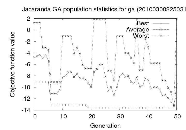
Figure 1: Statistics for population as it evolves under the control of a genetic algorithm
The commands to generate this plot are created automatically by Jacaranda and placed in the org-mode formatted output file.
External models in Jacaranda
Every object in the Jacaranda system can have a model associated with it. By default, these models are written in the Jacaranda Expression language. This language supports vector based arithmetic but is essentially a calculator. Sometimes, a more powerful modelling language is required.
Jacaranda has been extended to allow the use of external modelling systems. A framework has been put in place. At the moment, only one external language interface has been defined: for the GAMS modelling system. With this interface, a model can be written in GAMS and Jacaranda can communicate with GAMS to transfer values into GAMS and back out again.
A small GAMS modelling example
Consider the following Jacaranda input file:
use jacaranda.base

define
  variable x1upper 2.5	# this will be used to set a GAMS value below
end

EGO gamsmodel
  model gams
    code test.gms	# where the base gams model code is
    command "/opt/gams/22.8/gams" # how to run gams on this system
    # use x1upper Jacaranda variable to set GAMS variable X1.UP
    in x1upper X1.UP
    # and take result from GAMS of z and place in Jacaranda's z value
    out z.l z
    objective "solve test using nlp minimizing z"
    result z            # evaluate this expression to generate result
  end
  evaluatemodel		# do it!
  print
end
This example creates a simple object which defines the model
associated with the object as being an external GAMS model. The GAMS
model is in the file test.gms and includes everything but the actual
solve directive. The solve directive is specified by the
objective statement in Jacaranda.
The test code for this example is here:
$TITLE Test Problem
$OFFSYMXREF
$OFFSYMLIST

* Example from Problem 8.26 in "Engineering Optimization"
* by Reklaitis, Ravindran and Ragsdell (1983)
* Code from
* http://www.che.boun.edu.tr/courses/che477/gms-mod.html#TEST.GMS
* (from a course by Ignacio Grossmann)

VARIABLES X1, X2, X3, Z ;
POSITIVE VARIABLES X1, X2, X3 ;

EQUATIONS CON1, CON2, CON3, OBJ ;

CON1..  X2 - X3 =G= 0 ;
CON2..  X1 - X3 =G= 0 ;
CON3..  X1 - X2**2 + X1*X2 - 4 =E= 0 ;
OBJ..   Z =E= SQR(X1) + SQR(X2) + SQR(X3) ;

* Upper bounds
  X1.UP = 5 ;
  X2.UP = 3 ;
  X3.UP = 3 ;

* Initial point
  X1.L = 4 ;
  X2.L = 2 ;
  X3.L = 2 ;

MODEL TEST / ALL / ;

OPTION LIMROW = 0;
OPTION LIMCOL = 0;
The Jacaranda input defines a new value for the upper bound on X1
and the result of evaluating the model is the value of the z
variable, specifically the level of that variable, z.l. The in
and out directives specify how to bring values in to the model
from Jacaranda and then back out again.
The output from Jacaranda, in org-mode in Emacs, can be seen here:
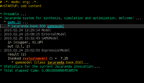
where we can see that the result of solving the GAMS model is 7.25.
This is actually a higher value than the optimum because we have
restricted variable X1 to a smaller upper bound, to illustrate the
transfer of values from Jacaranda to GAMS, and the optimum lies above
this upper bound.
The result can be any expression and not just a single variable. The
expression uses Jacaranda's own modelling language but has access to
any variables exported from the GAMS model (z.l in this case). Any
number of variables can be imported into the GAMS model and any number
exported as well.
The Genetic Algorithm classes
One of the built-in optimisation tools in the Jacaranda system is based on genetic algorithms. This short note describes the layout of the relevant classes and illustrates their use with a simple MINLP problem. The aim is not only to illustrate their use but also to explain how these classes can be extended or used directly to build new targeted genetic algorithm solution methods.
All classes and interfaces described in this section are in the
jacaranda.util.opt package unless stated otherwise.
The GA classes in Jacaranda
The following figure shows the three base classes which make up the genetic algorithm system. The GA class is the main controlling class. It will have a single population which must be provided during the definition of an instance of the GA object. The population will consist of a set of chromosomes, with the initialisation requiring the provision of a single chromosome to seed the population. The population may also be given diversity and selection objects which are discussed below. The chromosome is an interface; there is at least one base implementation, also described below, but it is through defining a new chromosome implementation that the method can be tailored for specific problems.
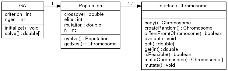
Figure 2: Base class hierarchy for the Genetic Algorithm procedure in Jacaranda
An implementation of the Chromosome interface,
VariableEncodedChromosome, is available in Jacaranda, suitable for
general MINLP (mixed integer nonlinear programme) problems. These
problems are defined by a combination of real and integer decision or
optimisation variables, one or more objective functions, possibly
constraint equations, both equality and inequality, and bounds on the
decision variables. This general Chromosome implementation is
actually more general than this and is suitable for any object that
can be encoded into and decoded from a combination of real and integer
variables but whose fitness can be evaluated through an objective
function object.
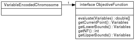
Figure 1: Variable encoded chromosome uses an objective function object for evaluation
The mate and mutate methods use appropriate operations for MINLP
problems. Specifically, the crossover operation is based on a
multi-point crossover across both real and integer variables. The
mutation operator selects on variable, randomly from the set of both
real and integer variables, and gives it a new value randomly from the
domain for that variable. These operators are actually implemented by
the Encoding implementation. The default encoding used by the
VariableEncodedChromosome is the GeneralEncoding class.
Alternative encodings include the BoundaryMutationEncoding, which
replaces the mutation operation with one which emphasises a move to
the boundaries for the selected variable, and the BinaryEncoding,
which encodes each real and integer value in a prespecified number of
bits for each variable.
The NLP and MINLP classes implement the ObjectiveFunction
interface and provide the ability to define the actual objective
functions (Jacaranda support multi-objective optimisation fully),
equality and inequality constraints and the lower and upper bounds on
the decision variables.
An MINLP example
 1	use jacaranda.util.opt
 2
 3	echo "----------------------------------------------- Objective function"
 4	MINLP model
 5	  # objective function with both real, x, and integer, y, variables
 6	  f "(x[0]-5)^2+(x[1]-3)^2-y*sqrt($x)"
 7	  # inequality contraints.
 8	  g "{ 2-(x[0]+x[1]), (x[0]+x[1])-10 }"
 9	  # lower and upper bounds
10	  a "{0, 0}" "0"
11	  b "{10, 10}" "1"
12	end
13
14	echo "----------------------------------------------- Chromosome"
15	VariableEncodedChromosome var
16	  function model
17	end
18
19	echo "----------------------------------------------- Selection"
20	RouletteSelection roulette
21	end
22
23	echo "----------------------------------------------- Population"
24	Population pop
25	  chromosome var
26	  crossover 0.75
27	  elite 1
28	  mutation 0.02
29	  n 20
30	  selection roulette
31	end
32
33	echo "----------------------------------------------- GA"
34	GA ga
35	  outputlevel 2
36	  population pop
37	  ngen 50
38	  solve
39	  print
40	end
Octave interface to Jacaranda
Octave can be used with Jacaranda for access to more powerful or specific optimisation and data analysis methods. A new interface for Jacaranda from Octave has been defined.
Introduction
An interface to Jacaranda from Octave (a tool similar to, and often very compatible with, Matlab) is potentially very useful, especially in the context of optimisation. Jacaranda provides a framework for process definitions, including simple or complex physical properties and processing units. Although Jacaranda has a number of optimisation methods included, it is not meant to be all-encompassing. As much of the optimisation research world-wide uses Octave or Matlab, an interface from Octave (due to its open source nature in preference to the proprietary and closed source Matlab) can be useful.
Previous versions of Jacaranda have included such an interface. However, the interface was based on the use of socket communication which could be slow when many objective function evaluations were required. It was also not a very portable solution which, although not often an issue (Jacaranda runs well on almost any Linux distribution), there is not reason to be limiting in portability.
Recently, a generic interface from Octave to Java has been implemented by Michael Goffioul. Jacaranda has therefore been updated to make use of this interface as it provides a much more elegant solution than what Jacaranda had before and is also more efficient.
An example
The full Jacaranda distribution (provided to collaborators) includes an input file which demonstrates this interface. As the more general distribution does not include this particular input file, I include it here for illustration:
 1	## Test out the Octave Java interface to Jacaranda.
 2	##
 3	## Eric S Fraga
 4	function jacaranda_test
 5	  persistent version;
 6	  if (isempty(version))
 7	    version = "2008.08.05 23:55:43";
 8	    printf ("ESF %s, Octave java to Jacaranda function evaluation\n", version)
 9	  endif
10	  ## initialise the Jacaranda interface from Octave, using a test input
11	  ## file which defines an appropriate objective function.  The
12	  ## particular example, from Rathore et al (1974) is the design of a
13	  ## heat integrated distillation sequence.  The input file will
14	  ## generate at least one flowsheet design.  This flowsheet will define
15	  ## an objective function with 8 real optimisation variables and 3
16	  ## criteria for optimisation.
17	  ##
18	  ## Note that the following assumes that the Jacaranda class files are
19	  ## stored in the given location relative to this file and that,
20	  ## therefore, Octave has been started in this directory.
21	  [A B nx ny nf] = jacaranda_init ("../vle/rathore_hen.in", \ # input file
22					   "rathore_hen-1-1", \	      # objective function
23					   "../../src/java")	      # Jacaranda classpath
24	  ## now evaluate the flowsheet at a number of random points
25	  N = 100;
26	  Y = [];
27	  n_infeasible = 0;
28	  for i=1:N
29	    x = A + rand(1,length(A)).*(B-A);
30	    try
31	      y = jacaranda_evaluate (x);
32	      Y = [Y; y];
33	    catch
34	      n_infeasible++;
35	    end_try_catch
36	  endfor
37	  if n_infeasible > 0
38	    printf ("There were %d infeasible design points (out of %d total) found.\n", n_infeasible, N);
39	  endif
40	  printf ("Minimum criteria values: %8.2e %8.2e %8.2e\n", min(Y));
41	  printf ("Maximum criteria values: %8.2e %8.2e %8.2e\n", max(Y));
42	  ## the results obtained above are plotted to give some indication of
43	  ## the variation in the three criteria for random design points
44	  plot (Y);
45	endfunction
I believe the comments describe clearly what is happening so I will leave it at this for now.
Defining simple unit models in Jacaranda
Simple unit models can be written using the Unit class in Jacaranda
with the equations written in the expr expression evaluator
available in Jacaranda.
Introduction
Although the Jacaranda system comes with a number of pre-defined process unit models (e.g. Distillation), there are many problems in conceptual design that only require simple models. These simple models may not require complex physical property values and may consist of, for instance, idealised mass and energy balances. For these cases, it may be worthwhile to define ad hoc simple models.
Jacaranda provides a generic model for such cases: units.Unit [1],
intended for use with streams supporting vapour liquid equilibria
properties (although methods for estimating specific VLE properties
won't actually be accessible).
Defining an actual model instance using this generic model consists of a number of steps: specifying the process streams that interact with the unit, definining design variables (to allow for analysis and optimisation), defining the equations that describe the unit operation, and defining the equations that can be used for analysis or evaluation (e.g. values used by the criteria definitions). These are described in detail below through the use of a simple example.
The example problem
The problem we wish to consider is the production of HF, as described
in Laing & Fraga (A case study on synthesis in preliminary design,
Computers & Chemical Engineering 21:S53-S58, 1997). Potential
candidate designs for the process need to consider a wide range of
units with varying degrees of detail. The units required include a
kiln (essentially a reactor), an acid blender, an absorber, a quench
unit and distillation. The distillation unit is modelled through the
detailed (albeit short-cut) model available in Jacaranda
(units.vle.Distillation) whereas the others can be represented using
simpler models.
Process streams
There are three types of streams which interact with process units: input (a.k.a. feed) streams, makeup streams (feed streams whose definition depends on the unit operation) and the outputs of the unit. Although makeup streams are really input streams, they differ from input streams in that they are defined as a result of the unit design. The specific input streams, however, will be specified to the unit before the design is attempted.
The kiln unit has one input stream, the main feed, two output streams, the gas stream which is vapour and is the main product of the unit and the waste stream which is in solid phase, and an air make-up stream, of known composition but with the flow rate to be determined by the design model:
use jacaranda.design.units
Unit kiln
  input feed
  output gas
  output waste
  makeup air air
The feed stream will be specified by Jacaranda prior to any design being attempted.
Output streams are created by the Unit model itself. The general
syntax of the output command is:
output NAME [TYPE]
where the square brackets indicate that the type of the output stream
is optional. If specified, this should be a class which implements
the ps.StreamExpressionInterface. If the type is not given, as in the
example above, the system will create a stream of the default type,
units.vle.Stream
The syntax for the makeup command is
makeup NAME INSTANCE
where the instance should be an actual stream which describes the composition of the makeup stream to be used. The amount or rate of that stream will be defined by the design model equations. The air makeup stream definition is
Stream air
  phase
    components O2   CO2    N2
    x          0.20 0.0325 0.7675
    vapour
  end
end
All streams, whether input, output or makeup, will have variables
available for use in the design equations. The actual variables
defined will depend on the stream definition. For the default base of
units.vle.Stream, the following variables are defined: F, the
amount or flow of the stream; x, the molar or mass composition in
fractions; P, the pressure in atm.; T, the temperature in Kelvin;
and, state, the state of the stream (0 is solid, 1 is liquid and 2
is vapour). For input streams, these variables are defined and set
before the design is evaluated; for output streams, the design
equations should give values to all of these variables as they will
then be used to define the actual output streams. For makeup streams,
the composition, x, will have been defined but all others will be
undefined and should be set by the design model.
Input stream checking
Before attempting a design, Jacaranda will query the unit model to see if the input streams specified are appropriate or not. In other words, the unit will be given a chance to indicate whether the feed streams assigned to the unit are suitable for that unit. The unit does this by specifying a set of conditions for the feed:
feedconditions LOGICAL_EXPRESSION
which, for the kiln example, looks like this:
feedconditions "feed.x[CaF2]>epsilon & feed.x[H2SO4] > epsilon"
This is using the feed input stream defined above and looks to see if
the stream contains any significant amounts of  and
and
 .
.
Heat transfer requests
Most units will require heating or cooling (or both). Requests for
heating or cooling are defined using the heat transfer request (HTR)
type in Jacaranda. Such requests are defined using the htr command:
htr NAME
which creates a set of variables for specifying the necessary
information for a heat request, much as stream variables are defined.
The components of a heat transfer request are Q, the duty (in kW with
negative values indicating that heating is required and positive
values indicating that the unit has an excess of heat so cooling is
required); T1, the inlet temperature for the process stream to be
heated or cooled; T2, the outlet temperature of the process stream;
and, U, the heat transfer coefficient  for the process stream side of any exchange.
For the kiln unit, we define:
htr heat
Design Variables
Design variables are variables which alter the behaviour or design of a unit. These variables are intended for Jacaranda to manipulate, either through the synthesis procedure or through generic optimisation methods within Jacaranda. For the synthesis procedure, it is sufficient to indicate that the variable is of type specification; for the general optimisation use, the variables must also be defined as tunable.
For the kiln unit, we define one such variable:
new specification "Single pass conversion of CaF2" RealSet conversion 0.95 0.96 0.97 0.98 0.99
The general format for defining a new variable is
new FUNCTION DESCRIPTION TYPE NAME VALUES
where FUNCTION is either specification or specification+tunable,
DESCRIPTION is a string which is purely decorative, TYPE is one of
Real, RealSet, Int, IntSet or Component, and VALUES describe the range
of values the variable should consider when used in either synthesis
or optimisation modes. For a RealSet variable, the values are a list
of discrete values. For other types, the values will be specified in
different ways. For instance, for the Real type, the definition would
look like one of the following:
new specification "Continuous design variable" Real x1 VALUE
new specification "Continuous design variable" Real x2 MIN MAX N
new specification "Continuous design variable" Real x3 VALUE MIN MAX N
In the first case, the variable is given the specified value and the
minimum and maximum values this variable can have are also this
value. This is not particularly useful for design (either for
synthesis or optimisation) but could be useful in debugging. The more
common case is the second where the definition says that ![$x_2 \in
\left [ MIN , MAX \right ]$](ltximg/jacarandablog_371d256bc6dcd655632be3f5e5ad99406a2e16a7.png) .
.
When using the synthesis procedures in Jacaranda, N indicates the
number of discrete values for this variable within the interval
specified. These discrete values will be uniformly distributed across
the interval, including both end-points if  . If a log
based distribution of the discrete points is required, one can use the
. If a log
based distribution of the discrete points is required, one can use the
LogReal type instead of Real.
The final case is the same as the second except that the variable is initialised to have the specific value given which may or may not correspond to one of the discrete values the system would normally use. This will not affect the synthesis procedures but will be useful for the process optimisation methods in Jacaranda.
Design Equations
When Jacaranda wishes to generate a design of the unit, it will
evaluate the equations given using the designequations command. These
equations are evaluated by the jacaranda.util.expr expression
evaluator. This is essentially a vector based calculator and does not
solve a system of simultaneous equations. If solving a complex system
of equations is required, the simple unit model is probably not the
approach one should take for defining the model. Alternative
approaches are beyond the scope of this short note so readers are
encouraged to approach the author for suggestions.
For the kiln model, the following are snippets of the equations we use with some commentary:
designequations
  # initialize the individual stream flows. we use the feed stream
  # composition vector to create new vectors of the correct size.
  gas.f = 0*feed.x
  waste.f = 0*feed.x
  feed.f = feed.F*feed.x	# feed stream individual component flows
The feed stream will have been defined by Jacaranda and the
appropriate variables (F, x, T, …) defined. These variables are
accessed by the stream name (as given in the input, output and makeup
commands above) followed by the full stop (.) and then the actual
variable name. The expression
feed.f = feed.F*feed.x
creates a vector of feed component flows based on the total flow, F, and the composition, x, of the feed stream.
# the air intake is directly related to the feed stream flow rate
air.F = air.ratio * feed.F
air.f = air.F * air.x
These equations define the actual amount of the air makeup stream
required. Recall that a makeup stream will have the composition
already defined.
# determine extents of reactions
extent = {0, 0, 0}
if feed.f[CaCO3] > feed.f[H2SO4]
   extent[0] = 0
   extent[1] = feed.f[H2SO4]
else
   extent[1] = feed.f[CaCO3]
   if feed.f[CaF2] > (feed.f[H2SO4]-extent[1])
      extent[0] = (feed.f[H2SO4]-extent[1])*conversion
   else
      extent[0] = feed.f[CaF2]*conversion
   endif
endif
if feed.f[SiO2] > (4*(extent[0]-feed.f[HF]))
   extent[2] = (feed.f[HF]+extent[0])/4
else
   extent[2] = feed.f[SiO2]
endif
These equations determine the extends of reaction. There are three reactions and it is important to note that the expression evaluator in Jacaranda uses a zero-based indexing for vectors.
Given the extents of reaction, the output streams can now be defined based on a simple extents of reaction mass balance procedure:
# now define the actual output stream compositions
gas.f[H2SO4] = feed.f[H2SO4] - extent[0] - extent[1]
gas.f[HF] = feed.f[HF] + 2*extent[0] - 4*extent[2]
gas.f[H2O] = extent[1]
gas.f[CO2] = extent[1] + air.f[CO2]
gas.f[SiF4] = extent[2]
gas.f[O2] = air.f[O2]
gas.f[N2] = air.f[N2]
gas.F = $gas.f				# total gas flow
gas.x = gas.f/gas.F				# and actual composition
gas.T = feed.T
gas.P = feed.P
gas.state = vapour
waste.f[CaF2] = feed.f[CaF2] - extent[0]
waste.f[CaCO3] = feed.f[CaCO3] - extent[1]
waste.f[SiO2] = feed.f[SiO2] - extent[2]
waste.f[CaSO4] = extent[0] + extent[1]
waste.F = $waste.f				# total waste stream flow
waste.x = waste.f/waste.F			# and composition
waste.T = feed.T
waste.P = feed.P
waste.state = solid
Note the use of the $ operator which means sum of all elements of the
vector to calculate the total flow of the gas and waste streams.
Given the specifications on the output streams, we can now design the actual physical unit. This includes a simple quadrature rule for evaluating an integral numerically:
# finally, design the actual reactor which is based on a numerical
# integration, as described above.
nsteps = 100
N = 2/3
M = 1/3
k450 = 0.247
E = 38363
k = k450 * exp(-1 * E * (1/feed.T - 1/450)/R)
Xf = conversion
Xo = preconversion				# preconversion
Rc = feed.f[CaF2]/(feed.f[CaF2]+feed.f[CaCO3])	# CaF2:CaCO3 ratio
Ra = (feed.f[H2SO4]-extent[1])/feed.f[CaF2]		# Acid:CaF2 ratio
dX = (Xf-Xo)/nsteps
rio = (1.0 - (1.0-Xo)^M) / ( k*(Rc*Rc*(Ra-Xo)*(Ra-Xo)*(1.0-Xo)^N) )
X = Xo + dX
t = 0					# residence time in minutes
while X <= Xf
  ri = (1.0 - (1.0-X)^M) / ( k*(Rc*Rc*(Ra-X)*(Ra-X)*(1.0-X)^N) )
  t = t + dX*(ri+rio)/2
  rio = ri
  X = X + dX
endwhile
volume = feed.F*t*60			# remember to convert to seconds
diameter = (volume*4/(Pi*htod))^(1/3)
height = diameter*htod
Finally, given the extents of reaction, we can solve the energy balance equations to tell us the amount of heating or cooling required. The numbers calculated are used to define a heat transfer request (HTR) which was defined above:
  # now calculate the heat balance; recall that Q for a heat
  # transfer request will have a positive value for cooling and a
  # negative value if heating is required so we need to negate the value
  # we get from the heats of reaction directly.

  # values in the next equation are heats of reaction [kJ/kmol]
  heat.Q = - extent*{53.7, 91.1, -189.4}
  heat.T1 = feed.T
  heat.T2 = feed.T
  heat.P = feed.P
  heat.U = 1
end # of design equations
Evaluation equations
Once the design has been generated, Jacaranda will evaluate the model equations which will typically be used to give values to the variables used to evaluate the criteria for comparing alternative process designs and for optimisation. These variables will be problem dependent. For the kiln model, the only variable we need is the capital cost of the unit:
  model
    capcost = 1917 * diameter^1.066
  end
end # of Unit kiln definition
[1] In this blog, class names are typically abbreviated by removing
the leading jacaranda.design. prefix. Unless otherwise
noted, all classes should have this prefix to be fully qualified.
The full example model definition
The complete model definition, comprising all the pieces described above, can be found here:
# -*- text -*-
#
# Unit model definition for the HF case study.
# Eric S Fraga
# $Id: kiln.in 2 2004-04-17 20:20:23Z ucecesf $

use jacaranda.design.units

# the air makeup stream used by the unit below
Stream air
  phase
    components O2   CO2    N2
    x          0.20 0.0325 0.7675
    vapour
  end
end

# The kiln is essentially a reactor. There are three reactions:
#
# CaF2 + H2SO4 -> 2 HF + CaSO4          Hr =   53.7
# CaCO3 + H2SO4 -> CO2 + H20            Hr =  -91.1
# SiO2 + 4 HF -> SiF4 + 2 H2O           Hr = -189.4
#
# The model is again essentially a simple mass balance. There are two
# product streams (HF off-gas and solid waste), one feed stream and
# one make up stream (air intake)
#
# The size of the reactor is estimated by first estimating the
# residence time based on the following model (from Laing & Fraga, 1997):
#
# -----------------------------------------------------------------
# Reactor Residence Time
# ----------------------
#  From internal report (see jwp)
#    dX/dt = r = k (Rc^2*(Ra-X)^2*(1-X)^N / (1 - (1-X)^M)
#
#   X = conversion of CaF2,
#   Rc = mol of CaF2 per mol of Ca in fluorspar feed.
#   Ra = acid:spar ratio
#   k = rate constant
#   N & M are constants dependent on rate model
#
#   The rate constant is given by
#     k(T) = k(450) exp(-E*(1/T -1/450)/R)
#
#   R = 8.3143 kJ/kmolK
#   Rate models :   N   :  M  : k(450) (min^-1X^-2)  : E (kj/kmol)
#      9          2/3     1/3      0.247                 38,263
#      10         1/3     1/3      0.166                 35,379
#
#  Use simpsons rule to integrate dX/r from prereactor conversion(Xo)
#  to final conversion (X).
#
# Use rate model 9, for the sake of argument!
#
# Note: residence time is in minutes!
#
# ----------------------------------------------------------------
vle.Separator kiln
  # make sure we can control the number of occurences of this unit
  limit
  new specification "Single pass conversion of CaF2" RealSet conversion 0.95 0.96 0.97 0.98 0.99
  new input "Reactor height/length to diameter ratio" Real htod 6.5
  new input "Pre-reactor conversion" Real preconversion 0.3
  new input "Ratio of air to feed" Real air.ratio 0.05
  output gas vapour
  output waste solid
  makeup air air
  htr heat
  #
  # must ensure that we have some CaF2 in the feed stream
  #
  feedconditions "feed.x[CaF2]>epsilon & feed.x[H2SO4] > epsilon"
  # now the design equations which include defining the extents of the
  # reactions and the actual sizing information for the unit
  design
    # initialize the individual stream flows. we use the feed stream
    # composition vector to create new vectors of the correct size.
    gas.f = 0*feed.x
    waste.f = 0*feed.x
    feed.f = feed.F*feed.x              # feed stream individual component flows
    # the air intake is directly related to the feed stream flow rate
    air.F = air.ratio * feed.F
    air.f = air.F * air.x
    # determine extents of reactions
    extent = {0, 0, 0}
    if feed.f[CaCO3] > feed.f[H2SO4]
       extent[0] = 0
       extent[1] = feed.f[H2SO4]
    else
       extent[1] = feed.f[CaCO3]
       if feed.f[CaF2] > (feed.f[H2SO4]-extent[1])
          extent[0] = (feed.f[H2SO4]-extent[1])*conversion
       else
          extent[0] = feed.f[CaF2]*conversion
       endif
    endif
    if feed.f[SiO2] > (4*(extent[0]-feed.f[HF]))
       extent[2] = (feed.f[HF]+extent[0])/4
    else
       extent[2] = feed.f[SiO2]
    endif
    # now define the actual output stream compositions
    gas.f[H2SO4] = feed.f[H2SO4] - extent[0] - extent[1]
    gas.f[HF] = feed.f[HF] + 2*extent[0] - 4*extent[2]
    gas.f[H2O] = extent[1]
    gas.f[CO2] = extent[1] + air.f[CO2]
    gas.f[SiF4] = extent[2]
    gas.f[O2] = air.f[O2]
    gas.f[N2] = air.f[N2]
    gas.F = $gas.f                              # total gas flow
    gas.x = gas.f/gas.F                         # and actual composition
    gas.T = feed.T
    gas.P = feed.P
    waste.f[CaF2] = feed.f[CaF2] - extent[0]
    waste.f[CaCO3] = feed.f[CaCO3] - extent[1]
    waste.f[SiO2] = feed.f[SiO2] - extent[2]
    waste.f[CaSO4] = extent[0] + extent[1]
    waste.F = $waste.f                          # total waste stream flow
    waste.x = waste.f/waste.F                   # and composition
    waste.T = feed.T
    waste.P = feed.P
    # finally, design the actual reactor which is based on a numerical
    # integration, as described above.
    nsteps = 100
    N = 2/3
    M = 1/3
    k450 = 0.247
    E = 38363
    k = k450 * exp(-1 * E * (1/feed.T - 1/450)/R)
    Xf = conversion
    Xo = preconversion                          # preconversion
    Rc = feed.f[CaF2]/(feed.f[CaF2]+feed.f[CaCO3])      # CaF2:CaCO3 ratio
    Ra = (feed.f[H2SO4]-extent[1])/feed.f[CaF2]         # Acid:CaF2 ratio
    dX = (Xf-Xo)/nsteps
    rio = (1.0 - (1.0-Xo)^M) / ( k*(Rc*Rc*(Ra-Xo)*(Ra-Xo)*(1.0-Xo)^N) )
    X = Xo + dX
    t = 0                                               # residence time in minutes
    while X <= Xf
          ri = (1.0 - (1.0-X)^M) / ( k*(Rc*Rc*(Ra-X)*(Ra-X)*(1.0-X)^N) )
          t = t + dX*(ri+rio)/2
          rio = ri
          X = X + dX
    endwhile
    volume = feed.F*t*60                                # remember to convert to seconds
    diameter = (volume*4/(Pi*htod))^(1/3)
    height = diameter*htod
    # now calculate the heat balance; recall that Q for a heat
    # transfer request will have a positive value for cooling and a
    # negative value if heating is required so we need to negate the value
    # we get from the heats of reaction directly.
    heat.Q = - extent*{53.7, 91.1, -189.4}              # values are heats of reaction [kJ/kmol]
    heat.T1 = feed.T
    heat.T2 = feed.T
    heat.P = feed.P
    heat.U = 1
  end # of design equations
  # cost model
  model
    capcost = 1917 * diameter^1.066
  end
  print
end

# add this unit to the list of units available for process flowsheet
# generation
edit globalData
  unit kiln
end
This model is copyright Eric S Fraga, all rights reserved. Distribution and use not allowed without his permission.