Professor Eric S Fraga
Centre for Process Systems Engineering
Department of Chemical Engineering
University College London (UCL)
London, UK
An object oriented framework for automated design (process synthesis), including support for simulation and optimization, has been developed and implemented in the Java language. This framework is known as Jacaranda and is based on the use of implicit enumeration which simultaneously generates and searches the appropriate superstructure. The method is able to generate process flowsheets with heat integration and recycle structures, and is able to handle under-specified problems as they frequently appear in early, conceptual design. Jacaranda, as well as subsequent process optimization procedures, supports multi-criteria optimization.
This document gives an overview of the whole package, intended for both users of the package and developers writing new models and tackling different kinds of problems. Emphasis is placed on the use of the Jacaranda system. The first half of the guide is intended for users of the system while the second half concentrates on the information required to develop new models for tackling new types of problems. This latter section provides a brief overview of the class hierarchy and gives links to the code documentation.
This document serves two audiences, users of the Jacaranda system for automated design and programmers wishing to develop new models for tackling new problems in design and optimization. As a result, some sections can be safely skipped if the reader is only interested in using the system. Readers intending to simply use Jacaranda should read this introductory section, the section describing the user interface for Jacaranda, including examples, and the installation instructions. Software developers will need to read the whole document however.
Automated process synthesis methods have been developed using a wide range of approaches including the use of heuristics, evolutionary methods, and superstructure approaches. We have developed an approach, based on implicit enumeration in combination with dynamic proramming techniques, which simultaneously generates and searches a superstructure. This approach is described elsewhere: see the reference section.
This document primarily describes the Jacaranda Java system for automated design which is part of the FiSH (Fully-integrated Synthesis/Simulation Hierarchy) system. The FiSH system makes use of miscellaneous support tools which are included in the distribution, including for instance tools for heat exchanger network synthesis, genetic algorithm development, graphics, etc. The system is distributed as a set of Java packages with the main entry point being the class uk.ac.ucl.che.esf.Main.
In what follows, there will often be links to the Java
documentation associated with each class in
Jacaranda. These links will be useful, especially for
software developers but also for users of Jacaranda
as the documentation will include information about the commands
available for each type of object in the system. Specifically,
he parseLine method in each class will have some
information about the text-based interface for working with
instances of that class. The main index for all of the classes
in the system is here.
Java, the object oriented language from Sun Microsystems Inc, is a portable language intended to provide the capability of writing programs once which are then able to be used on a wide range of hardware and software systems. Jacaranda has been written using the features available in the latest (at ime of writing) version of Java, version 1.6. Jacaranda will likely not work with older versions of Java. The latest version of Java can be downloaded, free of charge, from the Sun website.
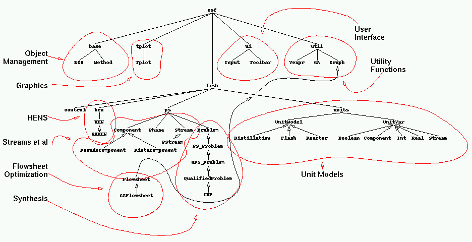
One of the features of the language, to ensure maximum portability, is the concept of packages, similar to the approach used in the Modula language. A package is a collection of classes and packages may contain other packages in a hierarchical manner. There is an old graphical representation of the full hierarchy of packages and subpackages (shown below in reduced size) in the distribution of Jacaranda rooted at uk.ac.ucl.che.esf.
|
| Annotated Hierarchy of the packages in Jacaranda |
Although this document is directed at explaining how to use Jacaranda, an understanding of some aspects of the Java packages is required. The distribution of Jacaranda contains a large amount of code written by the author while at the Department of Chemical Engineering in UCL (University College London) since 1996. The development of the majority of this code has been motivated by the research into synthesis methods. However, some parts are not directly related to synthesis yet are in the distribution of the package. This document does not aim to describe all the classes, concentrating instead on those relevant to process synthesis and the Jacaranda system.
The set of object classes for process synthesis are loosely grouped into a system known as Jacaranda. Jacaranda includes all the classes defined in the uk.ac.ucl.che.esf.fish.ps package. Jacaranda is not an acronym. Jacaranda also includes tools for process optimisation, typically applied after the synthesis step. These tools are mostly based on the use of stochastic optimization procedures, such as genetic algorithms and Simulated Annealing and are not described in this document. Further information can be obtained by contacting the author.
The synthesis procedures in Jacaranda are based on the use of discretization to convert the mixed-integer nonlinear programme (MINLP), used to describe a superstructure representation of a synthesis problem, into a discrete problem which can be described by a finite, albeit possibly large, directed graph. The optimization procedures use implicit enumeration to create this graph as it is traversed and result in ranked lists of N-best solutions. The best of these solutions is globally optimum with respect to the discretization parameters used.
At the core of the system are three classes:
 |
| Search graph |
The search graph, generated implicitly, has two types of nodes: Stream nodes and Unit design nodes. These correspond, in the state-task network view, to states and tasks respecively. In the graph, Stream nodes are reprented by boxes and unit nodes by boxes with rounded corners. Any stream node may have any number of edges emanating out from it. Each such edge leads to an instance of unit which performs some action on the stream. For example, the stream AD is shown being processed by a distillation unit which separates A from D and also by a reactor unit which converts A and B into C. The latter unit has an implicit make-up stream consisting of B.
Unit nodes have a number of edges equal to the number of outputs for the particular unit. For any given stream, there will be a number of unit designs, each of which differs in the operating conditions. These operating conditions are discretized by the underlying base unit model class, as described below. Likewise, he outputs of a unit are streams which are mapped to discrete space and therefore may lead to streams which are already present in the graph (eg. the outputs of left reactor unit and he distillation unit BC/D both lead to the same stream node, BC).
At the core of the Jacaranda system is the concept of discretization. All continuous quantities (e.g. component flows, unit operating conditions) are mapped to and from discrete space as appropriate. Developing new types of streams, in particular, requires specific attention to this aspect of the system, as will be described below.
The intention in developing the framework was to define a set of classes for the implementation of a generic solution procedure. As a result, the synthesis methods in Jacaranda are applicable to a wide range of problems, not limited to, for instance, phase equilibria problems. The system has been applied to problems in bioprocess synthesis (Steffens et al, 1999a,b) and for simple scheduling problems in brewing (Fraga et al., 1999). This last reference gives an overview of the generic object-oriented framework.
The stream, unit model and synthesis classes which form the core of the generic search procedures are described in more detail below. The rest of this section describes more general aspects of Jacaranda.
Underlying Jacaranda is the EGO class. All major classes in Jacaranda are subclasses of the EGO class. EGO provides basic functionality for the text input interface, the creation of persistent objects, and a rudimentary graphical interface. These aspects are all described in following sections, particularly in the input/output section.
In what follows, there will often be a reference to
expressions. These are algebraic expressions which are
evaluated by an instance of the uk.ac.ucl.che.esf.util.expr.Expression
object. The uk.ac.ucl.che.esf.util.expr.Expression
object is a fully capable expression evaluator, allowing the
definition of variables and the use of predefined functions
(such as trigonometric and exponential functions). All variables
are intrinsically vectors. However, the expression evaluator
does not solve systems of equations. It is essentially a
highly functional vector calculator.
Jacaranda comes with absolutely no guarantee or warranty, either
implicit or explicit. The software is provide as is and the user
should be aware that there may be errors in the code, as
distributed. The author takes no responsibility for the use of this
software. Please see the README and LICENCE files that come with the
distribution for further details.
The software is typical academic software in that it is intended for use as a test-bed for novel ideas in process synthesis and is not intended to be a production quality system. In particular, the user interface may not be as refined as one would like but it is suitable for the job intended. In any case, use this system at your own risk! Any and all comments, suggestions, bug reports and criticisms are most welcome.
Finally, the licence to use this software does not include the right to give copies to anybody else. If other people are interested in the software, please direct them to the author.
The main interface for the Jacaranda system is based on text input files. There is a graphical interface:
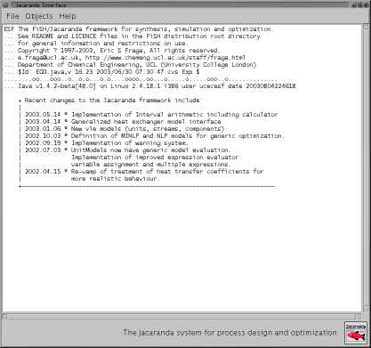 |
| Graphical interface for the Jacaranda system |
but this is only a simple interface to either input files or objects previously created using text input files.
The uk.ac.ucl.che.esf.Main= class is a simple front-end to the uk.ac.ucl.che.esf.ui.Input= class which is itself a simple Java based dynamic class loader. This provides an interface which allows objects to be created and modified. To use the text based interface, issue he command:
java uk.ac.ucl.che.esf.Main [options] input files...
This assumes that you have set your CLASSPATH environment variable correctly so that the Java virtual machine (JVM) can find the class uk.ac.ucl.che.esf.Main. See the installation instructions in the Appendix for more information on this. Alternatively, if you have the Jacaranda distribution in the form of a JAR file, you can run the system by executing the following command:
java -jar jacaranda-20020701.jar [options] input files...
where the 20020701 in the example above will vary as it is the date (in ISO format) of the release of the version of Jacaranda you have.
If no input files are given, the simple graphical interface is created and presented to the user.
The list of available options can be found interactively by
giving the '-h' option alone. Briefly, the options
available include:
window, the output is directed to a
graphical window that is created automatically.jacaranda.esfobjects in the user's home directory).
Note: make sure this directory exists before using this
option!The rest of the command line consists of input files which contain commands as described below. At the end of any invocation of Jacaranda which terminates normally (i.e. not interrupted by ^C), there is a summary of the run including an indication of any error or warning conditions that may have arisen.
The majority of the output generated by Jacaranda will be indented by 4 spaces. However, some lines will have some characters in the first three locations. The following cases are possible:
ESF ::
Indicates the dynamic loading of special Jacaranda
objects. Subsequent use of the same class will not be
flagged. The purpose of this line is to give an indication of
the version of the class, especially useful for reporting
errors to the author.
>>> ::
A new input file has been opened. Subsequent output relates
to this input file.
<<< :: The current input file has been read completely and
execution returns to the input file which redirected input to
the current file.
***DDDThere are two types of commands in the input files. The majority of an input file will consist of the definition of new objects. This is described below after a description of some special commands:
constant km " 1000*m"
will define the unit km using the predefined variable
mwhich defines the value of a metre.
feed.19980609195411.ucecesf.stream, where
ucecesf happens to be the author's userid. The date
is stored in ISO format (concatenation of year, month, day,
hours, minutes, and seconds). The second version of this
command is easier to use; it expects two arguments. The first
argument is the type of object and the second argument
is the name. This version will retrieve the most
recent instance of an object of the correct type and with the
given name, regardless of the user field.project command.name is an alias for this command.objects),
which must have been created prior to use of this
command. Alternatively, the user may specify given objects to
save by listing them on the same line. Each object is stored
in a file whose name is automatically created, as described
for the load command above.set
command enters a new command mode where the following are
valid (as in all other command modes, the end
command will terminate the mode):
'-s' option).#0.00. The format specification is based on the standard java.text.DecimalFormat. An example is #.0 which means any number of digits before the decimal place, including none, and only one and exactly one after the decimal place.#0.#.qfmt. Default value is #0.0.true or false indicates whether the system will allow the use of multiple threads when possible. Most users need not worry about this option at this stage.description.define command.Other than these special commands, the rest of an input file
consists of new object definitions. Each object definition
starts with a line which specifies the actual type of object
(the Java class) and a unique name to give the object created
from that class. Following this line comes a set of zero or
more lines which modify the contents of the particular object
created and finally a line with end on it alone. For
example, the following creates an instance, which we will name
propane, of the KistaComponent
class which is found in the uk.ac.ucl.che.esf.fish.ps
package:
uk.ac.ucl.che.esf.fish.ps.KistaComponent propane
  flow "45.36/10 * kmol/h"
  bp 230.8
  cpv -4.224 3.062e-1 -1.586e-4 3.214e-8
end
The flow, bp, and cpv commands are specific to the KistaComponent
class. Each class has its own set of commands and these are described
in the parseLine method every EGO object has. The class name has to
be a fully qualified Java name including the package hierarchy. The
only requirement on the type of object to be created is that it be a
sub-class of the uk.ac.ucl.che.esf.base.EGO class. The objects need
not be part of the Jacaranda system.
The definition of the flow value in the example above illustrates the
ability to use previously defined variables. The values of kmol and h
are previously defined; other variables, defined by the user, could
have been used in this example.
To make typing in the commands easier, the user can specify
default class paths to use when looking for the classes to
create new objects. This is done using the use
command. The example given above could be re-written as follows:
use uk.ac.ucl.che.esf.fish.ps        # specify class path directory
KistaComponent propane
  flow "45.36/10 * kmol/h"
  bp 230.8
  cpv -4.224 3.062e-1 -1.586e-4 3.214e-8
end
Interaction with the unit models is handled through the unit variables associated with each unit model. The list of unit variables for any unit model can be listed using an input file of the following form:
uk.ac.ucl.che.esf.fish.units.vle.Distillation
  print
end
where of course the first line is replaced by the actual class for the unit model of interest. See the sample output which would be generated by this sequence of commands.
The unit variables that can be modified by the user in an input file are those listed under 'General Unit Settings'. The 'Unit Design Specifications' may also be modified. The latter will be used by the Jacaranda synthesis procedure for generating unit design alternatives.
Unit variables are given new values by specifying the type of variable and the name of the variable followed (on the same line) by the value and optionally information describing the discretization parameters for the variable. Only variables which he unit model knows can be given new values. The commands above show how to find the list of variables that the unit recognizes. The type of variable must be consistent with the type expected by the unit model. For instance, if the unit model expects the particular variable to be a real number, then only types which generate real values can be used (e.g. Real, LogReal and RealSet).
The following input defines two unit variables as well as the equations used to evaluate the model after the design method has been successfully applied:
use uk.ac.ucl.che.esf.fish.units.vle
Distillation dist
  model
    V = 0.761*sqrt(1/P)
    diam = sqrt( 4*( 0.621*(1+RR)*D*sqrt($(mw*y)/(P/8.314/Tdd))) / Pi)
    height = 0.7 * ns
    colcost = msindex/280 * 101.9 * (diam/0.3)^1.066 * (height/0.3)^0.802 * 5.48
    traycost = msindex/280 * 4.7 * (diam/0.3)^1.55 * (height/0.3) * 2.7
    instrcost = 0
    maintcost = 0
    capcost = colcost+traycost+instrcost
    opercost = maintcost
  end
  LogReal    P  1 10 5
  Real       rec  0.98 0.98 1
end
The distillation unit model (in fact, all unit models) expects
the model to be a set of equations evaluated
sequentially (essentially, an expression calculator). The
equations can make use of variables defined earlier in the input
file and variables which the unit itself defines. All real
valued unit variables are automatically mirrored by expression
variables. For instance, the model equations listed above make
reference to the P variable (the operating pressure).
In the expression given in the example, the capital and
operating costs are defined by calculating the velocity of the
vapour in the column and the diameter and the height of the
column. The expression makes reference to example-defined variables,
such as the msindex variable, a global variable defined
by the system (but which can be altered by the user) and
variables such as RR and D which are defined
by the unit itself.
The first unit variable, P, is meant to be a real valued variable. The LogReal type defines a set of values uniformly discretized, on a log basis, between 1 and 10 atm. There are five values in the set. Finally, the recovery (rec) variable is given just one value. The operating pressure could have been specified as a Real variable or even a RealSet variable. The latter is particularly useful when one wishes to consider a diverse set of values for a particular variable. For instance, we may wish to have the synthesis procedure consider the design of distillation units with both low and high recoveries of the key components:
use uk.ac.ucl.che.esf.fish.units.vle
Distillation dist
  LogReal    P    1 10 5
  RealSet    rec  0.98 0.999  # consider two different recoveries
end
Please note that the use command must be used so that
the input parser can find the definition of the different unit
variables. In particular, if the unit variable types are to be
the standard ones in the package, the line
use uk.ac.ucl.che.esf.fish.units.vle
will be required somewhere above the definition of the units.
New unit variables can also be defined using the new
command. The syntax for this command is:
new TYPE DESCRIPTION SingleLineDefinition
where TYPE is one or more of input,
specification, tunable, and
continuation, concatenated with plus signs. The
DESCRIPTION is a general description of the variable in
double quotes, and SingleLineDefinition corresponds to
the syntax described above for single line re-definitions of
existing variables. A full example could look like:
new continuation "Continuation variable for optimization" Real theta 1
Some example input files are included as part of the standard distribution. These can be found in the examples directory of the documentation tree. Briefly, the following examples are available:
The first example above (rathore.in) will now be described in detail. It will be useful to refer to the document showing he input file with line numbers.
17  project Rathore
18  title "Separation sequence synthesis [Rathore et al., 1974]"
These two lines define the name of the project the input file
represents along with a one line description of the
project. This information is only used if you ask for an HTML
report to be generated (either via the report command
later in the input file or through the -r option on the command
line). The report will be created in a subdirectory (sub-folder)
given the name of the project.
24  use uk.ac.ucl.che.esf.fish.ps
25  use uk.ac.ucl.che.esf.fish.units
These lines tell the input parser that, for the rest of the
input file and any input files accessed thereafter, all objects
that are not given fully qualified class names will be looked
for in these packages. The second of these lines is necessary if
you intend to define any unit variables using the standard types
(Real, RealSet, Expression, etc).
30  variables
31          constant Base 10 "Percentage component flow discretization"
32          # define the flows of the components in the feed
33          constant Fpropane  " 45.36 *kmol/hr"
34          constant Fibutane  "136.08 *kmol/hr"
35          constant Fnbutane  "226.8  *kmol/hr"
36          constant Fipentane "181.44 *kmol/hr"
37          constant Fnpentane  "317.52 *kmol/hr"
38          constant FeedFlow "Fpropane+Fibutane+Fnbutane+Fipentane+Fnpentane"
39  end
We now define some variables which will be available to both the input that follows (including any other input files referenced by this input file) and to the unit models. In this particular case, we define the base discretization to use for component flows in the system. We will see the use of this variable (Base) below when we define the components. The rest of the variables are the flows of the components in the feed stream, as we shall also see below.
48  KistaComponent propane
49          base "Fpropane/Base"
50          bp 230.8
51          cpv -4.224 3.062e-1 -1.586e-4 3.214e-8
52          lhtc "0.583 *kW/m^2/K"
53          vhtc "5.0 *kW/m^2/K"
54  end
This is the first instance of creating a new object. In this case, we ask for an object, named "propane", to be created based on the uk.ac.ucl.che.esf.fish.ps.KistaComponent class. The base flow (the smallest amount of flow that will be represented in any stream) is defined using two variables defined earlier. The other two commands specify the 1 atm boiling point and the 4 coefficients for estimating the vapour heat capacity. The liquid and vapour heat transfer coefficients are also specified. All other physical properties required by VLE systems will be estimated from the values defined here.
87  Phase feedphase
88          comps propane ibutane nbutane ipentane npentane
89          x 0.05 0.15 0.25 0.2 0.35
90          flow "FeedFlow"
91          phase liquid
92  end
We now define a Phase object. The phase will consist of the five components given with a total flow and specified mole fractions. This phase will be used to define the feed stream:
97  PStream feed
99          add feedphase
102          prange "6.8 *atm" "6.8 *atm"
103          nstates 1
105          P "6.8 *atm"
109          map
110  end
The PStream object is used to represent multi-phase streams. In this case, we only specify a single phase, the feedphase object defined above. We then define the range of pressures that streams will be using in this problem. In this case, we only allow one pressure level (nstates) equal to 6.8 atm. The actual pressure of this stream is set to this same value. If any unit encountered during synthesis or simulation later on creates a stream which is at a different pressure, the pressure will be set to the nearest value in the set of discrete values defined by the prange and nstates commands. In this case, no matter what value the pressure of a stream may be given by a unit, it will be mapped to 6.8 atm. One should be careful in defining a synthesis problem that the ranges of pressures used by units be consistent with the range allowed for streams.
126  DiscreteUtilities utils
127      hot  "Steam @ 28.23 atm"    503.5 503.5 "5000 *W/m^2/K" "1.0246 / GJ"
128      hot  "Steam@11.22atm"       457.6 457.6 "5000 *W/m^2/K" "0.773824 / GJ"
129      hot  "Steam@4.08atm"        417.0 417.0 "5000 *W/m^2/K" "0.573203 / GJ"
130      hot  "Steam@1.70atm"        388.2 388.2 "5000 *W/m^2/K" "0.41796 / GJ"
131      cold  "CooldWater@32.2degC" 305.2 305.2 "500 *W/m^2/K" "0.0668737 / GJ"
132      cold  "Ammonia@1degC"       274.00 274.00 "500 *W/m^2/K" "1.65035 / GJ"
133      cold  "Ammonia@-17.68degC"  255.32 255.32 "500 *W/m^2/K" "2.96871 / GJ"
134      cold  "Ammonia@-21.67degC"  251.33 251.33 "500 *W/m^2/K" "3.96226 / GJ"
135  end
For evaluating flowsheets, we often need to estimate operating costs. A significant operating cost is based on the utilities required for cooling and heating. The DiscreteUtilities object is used to define a set of discrete utilities, each of which is for either heating (a hot utility) or cooling (a cold utility). The specification of each utility consists of inlet temperature, outlet temperature, the heat transfer coefficient, and a cost per unit of energy.
145  Distillation dist
146    Real P "6.8 *atm"
147  end
These three lines define a Distillation unit model. We accept the defaults for all the variables the unit has defined, except for the operating pressure. The default is to consider 4 discrete pressures, uniformly spread in a log basis in the range 1 to 32 atm. Instead of the default, we ask this unit to only consider a single operating pressure of 6.8 atm. This is consistent with the range of pressures we can represent in streams, as described above.
152  ProductTank pure
164    Expression spec "$(x>0.90)"
173    interesting           # interesting leaf node for n-best diversity
174  end
The product tank unit is used to define the allowable outputs of any process. The main specification is the expression which is used to determine whether a feed to this unit is a valid product stream. The expression can make use of several values (see the documentation for the ProductTank unit for a full list). In this example, the variable x, which is a vector of mole fractions, is compared to the value 0.9. The result is a vector of 0's and 1's, with 1's corresponding to the values in x which are greater than 0.9. Given that mole fractions must add up to 1, only at most one such element in the vector will meet this constraint. The $ operator returns the sum of the elements in the vector that results from the comparison. If the value is non-zero, this expression is assumed to return a true value. therefore, if any mole fraction has a value greater than 0.9, the specification will have been met.
The next line is necessary for the Jacaranda synthesis
procedure. In order to provide the user with some control over
the diversity of solutions returned by the synthesis procedure,
the user can specify which outputs of the process are
interesting. There must be at least one product tank
which has this property in order for the synthesis procedure to
return any useful results.
179  FeedTank feedTank
180    Stream feed feed
181  end
As well as product tanks, we need at least one feed tank. These lines define a feed tank which produces the stream defined earlier in the input file.
193  Criteria criteria
200    criterion Capital sum capcost "$" 0.0 "#,##0"
201    criterion Operating sum opercost "$/yr" 0.0 "#,##0"
202    criterion Annualized sum "capcost/2.0 + opercost" "$/yr" 0.0 "#,##0"
203  end
Synthesis procedures need a means of comparing solutions in order to
choose the best one. The comparisons are done using the criteria
specified. Jacaranda is able to generate multiple solution lists where
the solutions in each list are ranked according to different
criteria. In the example above, there are three criteria defined: the
capital cost, the operating cost, and an annualized cost where the
capital is assumed to be amortized over two years. The specification
of a criterion includes the name, the operation (either sum or max),
the actual expression (which for the first two criteria is given as a
single variable), the units of the criterion, the minimum value
expected, and finally the formatting information using the format
expected by Java's java.util.DecimalFormat class.
Any variable can be used so long as it is generated by a unit, either as a unit variable or as an expression variable. Heat exchangers are evaluated in the same manner and the model equations for these can be overridden as in the case of unit models:
HeatExchanger he
  model
    deltain = abs(T1in-T2out)
    deltaout = abs(T1out-T2in)
    eps = abs(deltain/deltaout-1)
    if eps < 4e-4
       lmtd = (1+eps/2-eps^2/12)*deltaout
    else
       lmtd = (deltain - deltaout)/log(deltain/deltaout)
    endif
    A = Q/U/lmtd
    capcost = 2000 + 35*A
    opercost = Cu*Q*h*hpy
  end
  print
end
This example replaces the default model by a better one which caters
for the difficulties that can arise when the inlet and outlet
temperature differences are the same. The model used here comes from
Morton (2002). Again, the variables available for use by the model
have been defined either in the global data object (e.g. hpy) or by
the HeatExchanger object itself (e.g. the area A). Again,
this other document shows the output generated by the print command
for the heat exchanger object, showing all the variables that are
available for use by the equation based model. In this case, it should
be noted that the global data object output includes the heat
exchanger model (as it is likely that one may have many heat
exchangers in a process, to reduce the amount of superfluous output,
the heat exchanger does not display its own model when using the print
command).
In the model, one specifies the expressions to evaluate to determine
the capital and operating costs. These expressions can use the
following variables: P, the pressure (atm) of the target stream, A,
the area ( ) of the exchanger, Cu, the cost of the utility
($/kW), and Q, the amount of utility (kW). Any other variables known
to the system can be used (such as hpy in the example above). The
capital cost is calculated before the operating cost so the capital
cost can be used in calculating he operating cost.
) of the exchanger, Cu, the cost of the utility
($/kW), and Q, the amount of utility (kW). Any other variables known
to the system can be used (such as hpy in the example above). The
capital cost is calculated before the operating cost so the capital
cost can be used in calculating he operating cost.
211  Data
212    utils utils           # which utilities object to use
213    criteria criteria     # the ranking criteria
216    unit dist             # distillation
217    unit pure             # and pure product tanks
218    unit feedTank         # and the feed tank
219    print                 # output all global settings
220  end
All general settings for the Jacaranda synthesis procedure are placed in a Data object. In this example, we can see how the set of utilities available, the criteria to use for ranking, and the list of allowable processing technologies have been defined. If we had wanted to include the new heat exchanger model defined earlier, we would have added the line:
hex he
to the Data object definition.
Given all the objects that we defined, we are now ready to attempt a synthesis problem. The synthesis problem definition for Jacaranda consists of the list of raw materials (represented by feed tanks in the list of units), desired outputs (product tanks in the list of units), and processing steps (the remaining units), together with the criteria for ranking. These have all been defined so we can now define and solve the actual synthesis problem:
236  PS_Problem rathore
237    representation units  # include unit info in n-best diversity
239    solve
240    print                 # and show the best solutions found
241    print short           # showing the basic structure as well
242    stats                 # display some statistics about the search
243    export                # generate the flowsheets
244  end
All the requirements for the problem definition have been given in the Data object. Therefore, all that remains before solving the problem is to specify any options that may be desired. In our case, we have asked that the representation of solutions include the unit id. The solution representation is a terse encoding of solution structures and is used to differentiate between different solutions when generating the list of best solutions. Two solutions that have the same structure, even if they differ in operating conditions, will not both appear in the list. The idea is to ensure that the list of solutions obtained at the end is as diverse as possible.
The next line actually solves the problem and the following
print commands output the solutions found . The stats command
displays some statistics about the problem size. The export
command generates flowsheet objects for each of the solutions
obtained. These will be named according to the name of the
problem object. In this case, the solutions generated will be
rathore-1-1, rathore-2-1 and
rathore-3-1. The first integer value is the criterion
and the second is the index in the list of solutions for that
criterion. By default, Jacaranda generates just one solution for
each criterion. This behaviour can be changed using the
-n option or by specifying nbest N in the
problem options (before the solve command).
As described above, the user can define new variables which may include new unit types. However, all values are stored internally and displayed to the user using the following set of units:
| flow | kmol/s |
| energy | kJ |
| length | m |
| mass | kg |
| power | kW |
| pressure | atm |
| temperature | K |
| time | s |
All output is based on these units (unless otherwise specified).
Input, if not qualified, is also assumed to be in these units.
However, all input can be given with units, as shown in the
examples in this document. If units are to be given, the
expression must be quoted and an operator (* or /) must precede
the units specified (this is a feature of the expression
evaluator used to parse the user's input). The following is a
list of known units for conversion (the full list can be
displayed using the print command within the
variables sub-mode described at the start of this
section): kmol, kg, kJ, kW, s, atm, m, K, mol, g, lb, hr, R (for
Rankin), bar, Pa, kPa, J, W, MW, GW, MJ, and GJ. Note
that case is significant.
Access to the package for the specific purpose of evaluating objective functions is provided through a client/server architecture. This is a limited interface to Jacaranda which provides the capability of executing previously prepared input scripts and the ability to evaluate objective functions at different points. The aim is to enable other software, specifically optimization tools, to use Jacaranda without writing any Java code. Access to any object which implements the ObjectiveFunction interface is provided. Access is also provide for objective functions which implement the ContinuationInterface for optimization with continuation methods.
The client/server implementation is only available in the full (source code) distribution of Jacaranda. If you have received the evaluation distribution, this interface is not available. If you require access to the client/server interface, please contact Professor Eric S Fraga.
The server is started using the command
java uk.ac.ucl.che.esf.Main --server
or
java -jar jacaranda-20020701.jar --server
remembering to replace the date code with the version given to you. These commands place the system in a wait state listening for connections to port 3817 (by default). Any tool can connect to the server through the use of sockets. Note, the implementation has been shown to work on Linux but no other systems have been tested at this point.
The remote or client application can access the server through a set
of function calls implemented in the C language. If you are intending
to use the client/server interface, you will need the full
distribution of Jacaranda (see below for installation instructions
which describe the difference in the distributions of Jacaranda
available). In this distribution, there are example files for
demonstrating the use of the client/serverb interface in C++
(example.cc), Fortran 90 (client.f90), and Octave (test.m). Remote
access from Java is provided by the RemoteObjectiveFunction class.
For Octave users, four functions are defined in the client code:
The octave files have to be installed in an appropriate directory (see installation instructions in this document and in the full source code distribution for more information). Once they are installed, and the appropriate environment variables defined, they should be accessible from Octave.
The rest of this document now explains the core object types that make up the Jacaranda system. Although it is not necessary to read the following in order to use Jacaranda, this documentation does explain the options available for the different units and also describes the different synthesis procedures currently available.
The core of the discretization procedure in Jacaranda is based on the Stream class. This base class is actually abstract, or what C++ programmers would call pure virtual. An abstract class is one which cannot be instantiated. These types of classes act as placeholders and the intention is that sub-classes of the abstract class will include the necessary implementation of what the abstract class promises.
Actual stream objects will be instances of subclasses of the Stream class. In the examples below, we will discuss the PStream class which works with Phases and knows about vapour-liquid equilibrium and related physical attributes. The base stream class need only provide an interface which is sufficient for the synthesis search procedure. This interface is described more fully in the class documentation; here we will concentrate on some of the most important aspects or methods:
The contents of the stream object are completely undefined and are left totally to the discretion of any subclass. The search procedure requires only the ability to map streams to the discrete space and to generate a string encoding of the stream. All else is up to the designer of the particular subclass. Below, we describe the PStream class which is used to represent streams for working with phase equilibria such as found in many synthesis problems in process engineering.
As mentioned above, associated with a Stream object is an object which implements the Composition interface. This is an object which describes, possibly more qualitatively, the composition of a stream and is used for recycle stream identification and for describing solution structures. It is up to the designer of the particular stream class to decide the level of detail that should be represented by composition object. The Composition object must implement the following methods:
An example of a Composition object is given in conjunction with the description of the PStream class.
Generating processes which involve, for example, distillation columns, requires us to have streams for which physical properties such as bubble and dew point temperatures can be estimated. The PStream can be used to represent such streams. It consists of one or more Phases at a given temperature and pressure. Each phase consists of a set of components and an amount, known as a flow (the time dimension is implicit in the amount and is assumed to be per second).
The Component objects implement the physical property estimation methods. In the current implementation, there are two different component classes: the KistaComponent class which uses Kistiakowski short-cut procedures for estimating physical properties from the 1 atm boiling point, and the PseudoComponent class which implements constant, user-provided, physical properties.
The PStream class uses the Phase object as its Composition. The composition object associated with a stream is a phase which is the combination of all the phases in the stream. Therefore, compositions for Streams, in terms of the search procedure, are described purely from the list of components in a stream, along with the amounts of each component. The temperature and pressure of the stream are ignored, as are the actual states of each phase.
Each Phase consists of a set of components. Each component has one basic quantity, a base flow, which is the basis for the discretization of streams. When a stream is mapped to discrete space, the component flowrates are mapped to the nearest integer multiple of the component's base flow. The pressure of a stream is mapped to the nearest pressure in a set of pressures defined by the user.
The second kind of node in the search graph corresponds to
processing technologies, as described by
unit models. Unit models, like streams, work in continuous space
but are used by the search procedure to define a discrete search
space. The search procedure takes one or more streams, maps them
to discrete space, and then passes them to a unit model
(UnitModel.setFeeds). The unit is then responsible for
deciding whether the feeds are appropriate and, if so, is given
a chance to prepare itself for use in a discrete search space
(UnitModel.prepareForAlternatives).
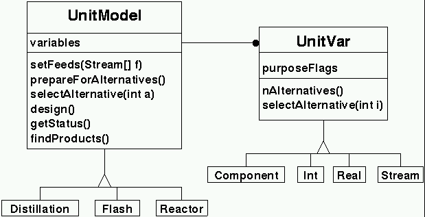 |
| Unit model class |
The only aspect of unit models that are directly used in the
mapping from continuous to discrete space is the set of unit
variables, describe using instances of subclasses of the UnitVar
class. The figure shows
the relationship between unit models and unit variables. When a
particular alternative design of the unit model is asked for
(UnitModel.selectAlternative), the base UnitModel class
determines which alternative from each of the unit variables is
required and these are chosen using the
UnitVar.selectAlternative method.
When a particular unit model alternative has been chosen, the
search procedure then requests the actual design using the
UnitModel.generateDesign method. This method invokes
the following methods:
preconditions command, valid for any unit model.constraints command.model command, also valid
for any unit model.If all these methods are successful, a unit design is available and the criteria can be evaluated.
The underlying rationale for the breakdown of a unit design generation
step into the sequence of method invocations described above is that
the user should be able to easily modify he default behaviour of a
unit model through the text input files. This is the reason for the
use of expressions for example-conditions, constraint checking and
model evaluation. The design method, however, is written in Java and
cannot be easily modified by the average user. Therefore, in
implementing any new unit models, care should be taken to ensure that
the design method be limited to only those actions that must be
undertaken in Java. An example is the direct interaction with the
stream objects for access to physical property estimation
methods. Another is the manipulation of the special unit variables
that are used by the synthesis procedures, such as the feed and
product streams and the heat transfer requests.
The search procedure interacts with the unit models both to create the search graph dynamically for the synthesis problem and to define diversity in the creation of multiple solutions (as described in the next section). There are two specific flags associated with unit models that affect the size of the search space and the types of solutions obtained:
true.The set of unit variables for a given unit model are used
directly by the search procedure, not only for mapping from
continuous space to discrete space, but also to identify
specific aspects of the unit design. Variables are given a
function when they are created and this function must be one or
more of the following (joined together using the OR
operator):
design method and is likely to include useful
information for displaying to the user.setFeed/setFeeds methods will automatically set
variables tagged with this function with the appropriate
streams.design
method, which will be addressed by the synthesis procedure
after a unit design. Heat transfer requests will result in the
design of heat exchangers, using either utilities or for
process integration.Tunable.The Jacaranda system provides a base unit model class which provides support for discretization and user input and output. Each unit model has a unit variable table which contains a set of unit variables. Each unit variable is described by a specific unit variable class which includes the type of variable and the method for discretization. Available unit variable classes include:
There are also array versions of many of these variables:
IntArrayUnitVar, RealSetUnitVar, StringArrayUnitVar, and
StreamArrayUnitVar. Each of these variables allows the system to
consider each entry in turn as different specifications for unit
designs (if the unit variable in question is actual a specification).
The user modifies the behaviour of unit models by specifying values and ranges for the different specification unit variables. Specifying values for unit variables is quite straightforward and is explained earlier. There are two types of unit variables the user will typically modify: design specifications and general settings. Design specifications are variables that are used by the synthesis procedure to generate the different design alternatives. These variables are often ranges of values. General settings affect the behaviour of the unit model but are not directly manipulated by the synthesis procedures.
The package provides an expression evaluator which is used by
some of the units. For instance, the spec and
valuefn product tank unit variables expect expressions
which are evaluated to determine, respectively, whether a stream
matches the product specification and the value of the any valid
product. In pure product separation sequence synthesis, for
example, the expression for the specification of a component
C1 could be defined as:
Expression spec "x[C1]>0.95"
One of the default variables defined for the product tank is the
vector, x, of mole fractions for the components in the
feed. The list of variables available for use is described by
each unit.
Jacaranda is distributed with a small set of representative unit models. These models are suitable for conceptual level design although their main purpose has been to enable the author to test the synthesis procedures. Although it is expected that users will develop their own targetted unit models, these models can and have been used. This section describes these models.
The distillation model (uk.ac.ucl.che.esf.fish.units.Distillation) implements a simple short-cut procedure based on the Fenske, Underwood and Gilliland equations. The model estimates the following:
This model also defines an expression for estimating the capital and operating costs which can be overridden by redefining the model unit variable.
The model requires certain specifications to identify suitable designs. The specifications understood by this model are listed here:
false will cause the model to calculate only the
minimum information for costing (number of stages and the reflux
rate) using only relative volatility calculations.rrf
value is used to choose the actual reflux ratio and this is then
used in the Gilliland correlation to identify the actual number of
theoretical stages.Given a feed stream, the light and heavy key components (which must be contiguous in relative volatility order), desired recoveries for the light and heavy keys, and a reflux ratio factor (explained below), the full design is generated.
The feed tank is used to specify the raw feed streams that are available to the system. As such, it has only one unit variable of interest: the feed stream.
The product tank unit is used to specify valid products of the process. These products are identified using expressions which describe valid compositions. The products can also have a cost associated with them. The variables of interest are
**cost**
design information unit variable and is hence accessible using the
criteria settings (described above).In tackling reaction/separation problems, it is often useful to introduce a purge unit. This unit will accept, as a valid feed to the unit, any stream which matches a desired recycle stream in terms of composition times some factor. The factor must be greater than 1. If this match succeeds, the purge unit " absorbs" the excess which is treated as an implied output of the process. The actual output of the unit is the stream which exactly matches the recycle stream.
The main purpose of including a purge unit in the synthesis procedure is to speed up the iterative procedure used by the iterative dynamic programming synthesis method. It is not typically necessary for convergence of that iterative procedure.
There is only one variable associated with this unit:
The reactor unit is very simple. The functionality one expects of a reactor unit is actually embodied in the uk.ac.ucl.che.esf.fish.ps.Reaction= class. The variables associated with this unit are:
As mentioned above, the reactor has a Reaction object associated with
it. See the class documentation for he reaction object for a more
detailed description. The reaction object to use with the reactor is
specified using the reaction command with a reaction object as the
argument. Although the reaction object is quite simple, the reactor
model can work with more complex reaction objects.
The main purpose of Jacaranda is the automated design of process flowsheets, or process synthesis. The Jacaranda synthesis procedure is embodied in the hierarchy of classes that start with the base Base problem and Solution classes. These classes provide the basic functionality for an implicit enumeration procedure which simultaneously generates and searches the appropriate graph describing the superstructure. The procedures use discrete programming techniques to implicitly define this graph and dynamic programming is used to make efficient re-use of computation. The basic procedures are described in the references.
The base problem class is not usable as it stands and is only meant to provide the basic framework for the search. Instead, subclasses are used to define specific synthesis problems; these subclasses are described below. A summary of the intended use of these problem classes is given here:
The first useful subclass of the base problem class is PS_Problem which stands for process synthesis problem. This class will typically be used for straightforward separation synthesis as it does not handle recycle streams nor can it generate heat integrated processes. The QualifiedProblem class is more general and can handle some of these aspects.
The definition of a process synthesis problem is based on the following information:
The PS_Problem class therefore requires this information to fully specify the synthesis problem. The user is expected to have defined a list of processing units, including at least one feed tank model (a unit with no feeds and one output) and one or more product tanks which are special units which have no output and which accept specific streams as feeds (e.g. a pure component product tank which accepts any stream with one component with a purity of at least 98%, say). The synthesis problem has default utilities (as described by Rathore et al, 1974). The list of units, utilities, and the exchanger models for heat exchange are all specified as part of the uk.ac.ucl.che.esf.fish.ps.Data global data object (see below).
The synthesis problem does have specific variables which control the behaviour of the search procedure and the types of results generated. The commands are available in the text based interface are listed here:
false as the argument, will turn off the
use of bounding in the search procedure.true if this behaviour is desired;
default is false.The Hierarchical synthesis procedure is used to generate and work with partial solutions. Partial solutions are those which violate one or more constraints, as specified in the problem definition. Examples can include flowsheets which have units that have cooling or heating requirements that can not be met by the current utilities or flowsheets which have streams which can not be processed any further and which do not meet the specifications for products (i.e. can not be accepted by any unit in the list of available technologies). These solutions, although infeasible, can be of interest to the user as they can give some insight into the problem and the corresponding search space. Furthermore, these solutions can be used by the QualifiedProblem subclass to automatically identify and generate recycle streams.
This class adds the concept of a status level to each solution. Solutions can now be compared not only with the cost, as done by the PS_Problem class above, but also with the status value. Status values are defined through a hierarchy of levels:
The default values can be modified by the user. It should be noted that the use of negative values (for example, to encourage product generation) is possible but should be used sparingly as bounding needs to be turned off in this case.
The generation of N-best solutions is handled differently by this
class. Instead of ensuring diversity only by the solution structure
(see the description of the representation option in the PS_Problem
class above), the HPS_Problem class defines diversity as a function
of the status value. The status value of any solution is the status
value of the root node plus the status value of the rest of the
flowsheet (recursive definition). For each different status value,
there will only be one solution. It is possible to change this
behaviour to allow multiple solutions with the same status value to
appear in the N-best list by using the differby command
with the argument structure (the default behaviour is
achieved by specifying status instead).
The QualifiedProblem class allows the user to specify certain qualities that the solution to the problem should observe. These may be extra restrictions (for example, a limit on the number of occurences for a particular unit such as a reactor) or they may provide extra resources specific to the problem (extra feeds, say). These are specified using Qualifiers; this section describes those that are currently available in the Jacaranda system.
limit flag set (see the description
of Unit models above).VHL :; To tackle heat integration, the system provides a special qualifier which implements the virtual heat links, described by Fraga & McKinnon (1994; 1995; & 1998).
Problems whose solutions require recycle streams are handled using the iterative dynamic programming class. This class is essentially the same as its superclass, the QualifiedProblem class except that the ability to iterate on partial solutions has been added. The procedure is described by Fraga (1998).
Some new commands are introduced in this class which affect the iterative procedure:
The synthesis procedure is based on ranking solutions according to user specified criteria. The default is to use the total annualized cost of the process as the sole criterion. The annualized cost is calculated as the capital cost divided by the plant life (default of 10 years) plus any operating costs. Capital costs come from the units and any heat exchangers; operating costs also come from the units (e.g. some units may require make-up streams or catalysts etc) and from utility consumption for heating and cooling. Other ranking criteria could include measures on dynamic behaviour such as maximum deviation from product specifications and response time.
Criteria are specified by creating an instance of the uk.ac.ucl.che.esf.fish.ps.Criteria
class. This class allows one to specify as many criteria as
required. Each criterion consists of a name, the operation to
perform to combine criterion values from different sources
(units, heat exchangers, subproblems) which can be either
sum or max, and the actual expression to
evaluate for the criterion. Optional extra arguments are the
units (e.g. $/y), the minimum value expected (which can be used
by bounding procedures in the synthesis algorithm to reduce the
size of the space searched), and the formatting instructions for
output of values for the criterion. The expression for each
criterion may make reference to any of the variables defined by
the various unit models and the heat exchanger models. The
latter only define capcost and opercost.
The following example defines three ranking criteria: the first is the capital cost, the second the operating cost, and the hird is a combination of the two where we assume we amortize he capital cost over 2.5 years.
use uk.ac.ucl.che.esf.fish.ps
Criteria  multipleCostCriteria
  criterion Capital sum capcost
  criterion Operating sum opercost
  criterion Annualized sum "capcost/2.5 + opercost"
end
(See the section on text input for a further description on how
input files are created and used.) This example creates an instance
of the Criteria class which is called
multipleCostCriteria. This instance is passed to a
synthesis problem through the global data object, described in the
next section. The data object has a command called criteria
for specifying the criteria object to use in ranking.
In the example shown above, it is assumed that the objective
function is equivalent to the sum of the annualized costs of all the
constituent parts of the process flowsheet (i.e. sum of unit and heat
exchanger costs). However, some measures correspond to objective
functions which find the maximum value of some criterion. Each
criterion expression for a Criteria object can be assigned the
operation that should be performed. At time of writing, only two
operations are allowed: sum and max.
Operations are defined using the operator command in the
text interface. If this command is not used, the operation for each
expression element defaults to sum.
Although the criteria object allows one to select the criteria
to use in ranking alternative solutions, this object does not
necessarily allow on to specify how the individual variables
used in evaluating criteria are calculated. For instance,
although the default criterion for ranking is based on the
annualized cost using the opercost and capcost
variables, no mention has been made of how these variables are
defined.
Costs come from two sources: processing units and heat exchangers
(where applicable, of course). All unit models define two types of
variables, the so-called Unit Variables and Expression variables. The
unit variables have names and any of these, assuming they correspond
to real values, can be used in the criteria expressions. For
instance, the Distillation unit model defines the operating pressure,
P. The expression variables can also be used and, in the case of the
Distillation model, variables such as diam and height are defined. The
full list of variables, both unit and expression, for any unit can be
listed using the print command in an instance of that unit. For
example:
use uk.ac.ucl.che.esf.units
Distillation dist
  print
end
will show something like this:
ESF Input: use uk.ac.ucl.che.esf.fish.units
ESF Input: Distillation dist
003 defining dist, a new unit
Distillation: print
ESF Object dist:
|
|   ---- Unit dist: Short-cut Distillation unit based on FUG ----
|
| type=unit
|         constraint: null
|        interesting: false
|              limit: false
|  post-design **model**: V = 0.761*sqrt(1/P)
diam = sqrt(4/(Pi*V)*(RR+1)*D*22.2*Tdd/273.0/P)
height = 0.61*S+4.27
colcost = (1+(P>3.4)*(0.0147*(P-3.4))) * (4.23*msindex/280.0*7620*diam*(height/12.2)^0.68)
raycost = 0.61*ns*msindex/280*111.41*(diam/1.22)^1.9
instrcost = 4000
maintcost = 0
capcost = colcost+traycost+instrcost
opercost = maintcost
|      **preconditions**: (F>minflow)
|             status: null
|
|   ---- Unit Design Specifications ---
|
| Light Key for Recovery: key undefined, expects Component.
| Operating Pressure [atm]: **P** = 1.0, real value in range [1.0,32.0] with 4 values log-uniform.
| Recovery of keys: rec = 0.98, real value in range [0.98,0.98] with 1 values.
| Reflux rate factor: rrf = 1.2, real value in range [1.2,1.2] with 1 values.
|
|   ---- General Unit Settings ---
|
| **minflow** = 0.0 (Minimum feed flow allowed)
| minx = 1.0E-8 (Minimum key mole fraction allowed)
| te = 1.0 (Tray efficiency)
| Use Eduljee correlation for actual stages: eduljee = false
| Conceptual mode: conceptual = false
| Saturated feed assumption: sfa = false
|
|   ---- Unit Feeds ---
|
| Feed stream to unit: feed = undefined, type Stream expected.
|
|   ---- Unit Outputs ---
|
| Top product stream: tops = undefined, type Stream expected.
| Bottom product stream: bottoms = undefined, type Stream expected.
|
|   ---- Unit heat transfer requests ---
|
| Cooling performed by condenser [kW]: Qc = undefined, expects a heat transfer request.
| Heating performed by reboiler [kW]: Qr = undefined, expects a heat transfer request.
|
|   ---- Unit Design Information and Other Variables ---
|
| ns = 0 (Number of stages)
|
|   ---- End of Unit Variables ----
|
|
| +-- List of local expression variables:
| | variable B =  0.0  (Bottoms flow rate [kmol/s])
| | variable D =  0.0  (Distillate flow rate [kmol/s])
| | variable F =  0.0  (Feed stream flow rate [kmol/s])
| | variable P =  0.0  (Operating Pressure [atm])
| | variable Qc =  0.0  (condenser duty [kW])
| | variable Qr =  0.0  (reboiler duty [kW])
| | variable RR =  0.0  (Reflux ratio)
| | variable S =  0.0  (Number of stages)
| | variable Tbb =  0.0  (bottoms bubble point temperature [K])
| | variable Tbd =  0.0  (bottoms dew point temperature [K])
| | variable Tdb =  0.0  (distillate bubble point temperature [K])
| | variable Tdd =  0.0  (distillate dew point temperature [K])
| | variable V =  0.0  (Velocity of vapour in column [m/s])
| | variable capcost =  0.0  (Capital cost of unit (column, trays & instrumentation) [$])
| | variable **diam** =  0.0  (Diameter of column [m])
| | variable height =  0.0  (Height of column [m])
| | variable instrcost =  0.0  (Cost of instrumentation [$])
| | variable minflow =  0.0  (Minimum feed flow allowed)
| | variable minx =  0.0  (Minimum key mole fraction allowed)
| | variable ns =  0.0  (Number of stages)
| | variable opercost =  0.0  (Operating cost of unit (maintenance) [$/y])
| | variable rec =  0.0  (Recovery of keys)
| | variable rrf =  0.0  (Reflux rate factor)
| | variable te =  0.0  (Tray efficiency)
| | variable traycost =  0.0  (Cost of trays [$])
| | variable x =  0.0  (Bottoms mole fractions)
| | variable y =  0.0  (Distillate mole fractions)
| | variable z =  0.0  (Feed mole fractions)
| +--------------------------------------------
+------------------------------------------------
Distillation: end
ESF Input: end
where some of the variables and unit settings that are relevant
have been highlighted in bold text. For instance, the
model expression used after a unit design defines the
capcost and opercost variables. These could
therefore be used in a criterion for ranking solutions. Also
highlight, by way of example, are the minflow unit
variable and the diam expression variable. The first is
used in the unit's preconditions expression and the latter is
used in the estimation of the capital cost.
Note that all the expression variable values in the example above are 0. This is because the design method has not yet been invoked.
To change the cost correlations, one need only change, in this
case, the expression defined for the model. One can
also change the actual criteria used for ranking, as described
earlier.
[[api/uk/ac/ucl/che/esf/fish/ps/HeatExchanger.html][Heat
exchangers]] are slightly different. Two special commands are
defined for these: capcost and opercost, each
of which expects an expression. These expressions are evaluated
to define the corresponding variables which can then be used in
the ranking criteria. There is no generic definition of criteria
for heat exchangers so capital and operating costs are all that
can be used. Of course, if a more complex cost correlation for
heat exchangers is required, the user has the option of defining
a new heat exchanger class. The system can be informed of the
new class by using the hex command of the uk.ac.ucl.che.esf.fish.ps.Data
object.
The synthesis procedures described above, as well as post-synthesis tuningmethods, rely on some data which is global to the system. This includes the list of units available for processing (including feed and product tanks), the utilities which can be used for meeting the heating and cooling requirements of units designed, the heat exchanger models, the criteria used for ranking solutions, as well as an assortment of values for cost models and the like. All of these global data are stored in a special object, uk.ac.ucl.che.esf.fish.ps.Data. Defaults are provided for, in particular, the criteria for ranking (total annualized cost based on a 10 year plant life) and utilities (discrete set based on those described by Rathore et al.).
This section describes some hints for improving performance. Basically, the following is a description of the main user-customizable factors which affect the performance of the synthesis procedures.
The search space size is primarily a function of the discretizations: the finer the discretization, the larger the search space and hence the longer the synthesis procedure akes. Initial runs should always use a fairly coarse discretization to ensure that some results are generated quickly, giving the user a feel for the type of performance to expect and possibly some feel for the results that are possible. Secondary effects on performance are found from the bounding and the size of the best solution list to present at the end. Bounding should always be turned on, unless the problem includes negative costs (such as product tanks which give a value for the product stream). The larger the number of solutions to present, the less effect bounding will have, however.
Another effect on performance, and possibly on the size of problem that can actually be tackled, is the amount of memory required. The memory needs are directly proportional to the number of solutions in the N-best list because a large amount of the memory requirements are the cost & solution table needed by the dynamic programming aspects of the search procedure. A secondary effect is the increase in search space as a function of N, due to the reduction in pruning from bounding. The use of multiple criteria has the same effects.
By default, unit designs are saved. For large problems, this can have a dramatic effect on memory use as well so, if the problem class is HPS_Problem or a superclass of it, turning off this feature may result in significant reductions in the memory usage.
The result of the synthesis procedure is implicitly defined in the solution structure encoded in the dynamic programming able. This structure is not immediately useful so the Jacaranda system provides a class for representing flowsheets. This class is able to extract the information from the solution structure to create a flowsheet representation; alternatively, the user may build up a flowsheet directly specifying units, feed streams, and the connections between them. The commands understood by the flowsheet objects are as follows:
FeedTank units. The example
creates a flowsheet with one feed stream, one distillation column,
and two outputs. A special command in this mode is utils
which is used to specify the utilities to use in evaluating the
flowsheet.export command defined for all
Problem classes. This automatically generates flowsheet
objects for each solution in each criterion list.Flowsheet objects implement the ContinuationInterface and the ObjectiveFunction interfaces. Flowsheet objects can therefore be used by the different optimizers in the Jacaranda system, such as the generic genetic algorithm and simulated annealing implementations. Through the client/server interface, optimization tools written in almost any other language can interface with Jacaranda for process flowsheet optimization. A recent paper (Fraga & Zilinskas, 2002) used a variety of direct search optimizers implemented in Matlab (actually Octave) for heat integrated process optimization.
Jacaranda provides the capability of saving EGO based objects for later use. Instances of saved objects are said to be persistent. All subclasses of the EGO class automatically inherit the ability to be saved and loaded from external storage. This ability is provided by the object serialization features introduced in Java version 1.1.
Both saving and loading objects are taken care of by the input/output interface in use, be it the text based interface which reads in commands from files or the graphical object viewer interface which allows the user to browse through a collection of previously saved objects (in the future, it should be possible to graphically create and manipulate new objects instead of only accessing previously created ones). How and where objects are stored or retrieved from is controlled by the browser, described in the next section.
Associated with any instance of Jacaranda (in a single Java Virtual Machine) is a browser (badly chosen name but it's historical... a better name would have been something like manager but this name is reserved for the graphical browsing tool. If you think you're confused, you should see what I'm like these days!). The browser is the link between the object system and the file system (if running the application version of the package) or between the objects and the remote file system (if running through a Web browser; it should be noted that at this moment the remote browser does not support saving objects).
The user does not typically need to worry about the browser. In
particular, when used through a Web browser, it's not really possible
to do anything different than what the system does by default. When
used from a standalone application, however, the user can have control
over which directory is used for object storage and retrieval. By
default, the local file browser works with the esfobjects
sub-directory from where the program was started or, on Unix systems,
the esfobjects sub-directory in the home directory. This can be
changed within an input file by specifying a different location:
directory NEWDIR
This will create a new local file browser associated with the directory specified and all further persistent object actions will refer to that directory.
Saved objects can be later accessed either through the text based
interface (using the load command) or through the
graphical interface (uk.ac.ucl.che.esf.ui.Manager).
The one issue that may lead to some confusion in the use of persistent objects is how the global data settings are handled. All global settings used by the synthesis and simulation aspects of the Jacaranda system are embodied in the uk.ac.ucl.che.esf.fish.ps.Data= object. Saving any object does not automatically save the global data settings. Reloading a previously saved object will use the current global data object settings. Therefore, if consistent results are desired (which is what is typically wanted, I guess), an instance of the global data object should always be saved and restored when associated flowsheet, for example, objects are saved and restored.
There are two different distributions of Jacaranda:
jacaranda and will include the date in ISO format (YYYYMMDD) indicating the date the distribution was made. The class files (i.e. the compiled executable version of the Jacaranda system) are in the JAR file and will have a name similar to jacaranda-20020701.jar or jacaranda-evaluation-20020701.jar. To use this version, simply execute the commandjava -jar jacaranda-20020701.jar [options] input files...
You may, of course, use the Java
jarcommand to extract all the files. This will create a subdirectory (subfolder) calledukand subdirectories within there. To use the system once extracted, you will need to point yourCLASSPATHvariable to the directory in which you extracted the contents of the jar file. So, for instance, the following sequence of commands would be suitable on Linux for extracting the class files and then running Jacaranda:
mkdir Jacaranda
cd Jacaranda
jar -x jacaranda-20020701.jar
export CLASSPATH=".:`pwd`"
java uk.ac.ucl.che.esf.Main [options] input files ...
If you have also received other supplementary files with this distribution, these will be in
zipformat. There should be extracted into theJacarandadirectory created in the example above. The supplementary files include the documentation (called something similar tojacaranda-doc-20020701.zip) which will be placed in thedocsubdirectory, a large number of sample input files (jacaranda-inputs-20020701.zip) in theinputssubdirectory, and the Java and JavaCC source code for the system (jacaranda-src-20020701.zip) in theuksubdirectory. Again, on Linux, we would execute the following command, assuming you received all the supplementary files.
unzip jacaranda-doc-20020701.zip
unzip jacaranda-src-20020701.zip
unzip jacaranda-inputs-20020701.zip
It is recommended that the documentation, which includes this file, be extracted in this manner. When extracted, all the links to the class documentation in this document are available if you use your browser to look at the file
doc/guide.html.
Extracting all the supplementary files will required approximately 16 MB of space.
jacaranda.tar.gz. Instructions on extracting and building the system are available in the INSTALL file which accompanies the full distribution. A summary of the instructions found in that file is given here:
Extract the files by issuing the commands
cd BASE
gunzip -c fish.tar.gz | tar xf -
Then change into the
fishsub-directory and modify theMakefilefound there to reflect the installation directory (you need to change the BASE variable defined near the top of theMakefile).
Compile the system, including both the Java packages and the client interfaces for the client/server implementation (described below) by
cd BASE/fish
make
and, optionally, install the client interface codes:
cd BASE/fish/src/server
make install
The BASE directory is where you would like to extract the FiSH system into. The string BASE should be replaced in the commands shown with the desired location. In step 3, the Java package should compile with no errors although there may be some warnings about deprecated methods depending on the version of Java you have installed on your system. These warnings are not serious and relate to part of the system that is currently not used, or is used for aspects which are not critical to the operation of the overall system. Jacaranda should run under versions of Java from 1.4 (released in early 2002) upwards.
This document refers, hopefully, to the latest version of the Jacaranda system. The numbering of the versions reflects the ancestry of some of the basic ideas. The immediate precursor to the Jacaranda system was the CHiPS process synthesis package (written in C and Fortran at the University of Edinburgh) although all the code in the Jacaranda system is new. The last development version of CHiPS was numbered 11 so the first version of Jacaranda started as revision 12. What follows is a brief description of the main changes or features in each major version.
It should be noted that recent distributions of Jacaranda, particularly as jar files, now come with a date as part of the name of the distribution. This date should be referred to in all communication with the author of the package so that he can help identify whether any problems you may be having have been rectified in a later version.
At this point, I would like to mention some of the more important restrictions or limitations in the current version of the software:
-3^2 evaluates to 9 instead of -9. To get the correct precedence, use parantheses, as in -(3^2).In summary, most of the author's effort to date has been on the actual synthesis procedures. All other code has been generated to help with developing the synthesis methods. In the future, however, it is envisaged that work will be devoted to improving links between the Jacaranda system and any open software in the flowsheeting area that appears (due to work in the CAPE.OPEN and Global CAPE.OPEN groups, for instance). Until then, the post-synthesis features will continue to be relatively primitive in comparison to the synthesis procedures.
The following are some of the articles referenced in this document. A full list of the author's publications can be found on his web site.