Joint Modelling of Functional and Structural Connectivity

A Gaussian Graphical Model

As the number of regions grows, it becomes more difficult to estimate a precise, well-conditioned covariance matrix. Well-conditioned refers to the intrinsic property of the correlation matrices to have positive eigen values. This is of paramount importance for the inversion of the correlation matrix to derive the partial correlation matrix. To obtain a better-conditioned covariance matrix the time-series are modelled based on Multivariate Autoregressive Models (MAR). MAR models interregional dependencies within the data, taking in consideration the time influence one variable has on another. This is different from regression techniques that quantify instantaneous correlations. Here, we consider the functional brain activity as a stationary process and we use a zero-lag MAR model:

$mathbf{F}=(mathbf{I_n}-mathbf{T})^{-1}mathbf{E}$

$mathbf{F} in mathbf{R}^{ntimes t}$ ,

is the number of regions and

the time points corresponding to the fMRI volumes. $mathbf{T} in mathbf{R}^{ntimes n}$ is a matrix specifying the connections between variables that can be understood as transition probabilities that reflect conditional independence. $mathbf{I_n}$ is the identity matrix and mathbf{E}

is Gaussian noise. Stationarity implies that the distribution of the signal does not change with time and therefore has similar mean and variance over time.

Gaussian graphical models provide a graph representation of relations between random variables. Here we represent the interrelationship between fMRI time-series as a undirected graph with

nodes/components representing the average fMRI signal within a set of

regions. The graph edges describe conditional independence relations between the nodes. The conditional independence relations between components correspond to zero entries in the inverse covariance matrix, precision matrix. Specifying the graph topology of a Gaussian graphical model is therefore equivalent to specifying the sparsity pattern of the inverse covariance matrix. Estimation methods for Gaussian graphical models extend to solving autoregressive Gaussian processes.

To restrict the topology of the Gaussian graphical model and reduce the number of parameters, we inject prior knowledge based on the structural data. Recall that in the partial correlation context the absence of a structural connection corresponds to absence of the corresponding functional connection. We can select which connections to remove based on a t-test on each structural connection across the overall population of subjects.

Functional Connectivity as a Multivariate Object

The geometrical interpretation of a symmetric positive definite (SPD) matrix is simple when we consider two dimensional covariance matrices. Let say that a set of 2D points is given. Second order statistics describe their location with an ellipse (ie. PCA). The long axis of the ellipse is in the direction of the highest variance. The short axis is in the dimension of the lowest variance. The eigenvalues of the system correspond to the long and short axis of the ellipse. Therefore, it is not meaningful to have negative values.

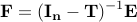
Note that the prediction of each functional connection independently results in an unconstrained matrix that does not represent correlation. This results in a system, which is underpowered to detect interactions between function and structure over several regions. We suggest to decompose the precision matrix:

$mathbf{Sigma}^{-1}=mathbf{B}^top mathbf{B}$

This cholesky decomposition results in a matrix mathbf{B}

that we can use for prediction, so that the reconstructed matrix mathbf{C}

is always SPD. It turns out that mathbf{B}

is the interaction matrix, which is also related to the connectivity matrix, $mathbf{B}=(mathbf{I_n}-mathbf{T})$ .

$mathbf{Sigma} = frac{1}{t}mathbf{F},mathbf{F}^top = (mathbf{I}_n-mathbf{T})^{-1} covmathbf{E},(mathbf{I}_n-mathbf{T})^{-mathsf{T}} = bigl((mathbf{I}_n-mathbf{T})^top (mathbf{I}_n-mathbf{T})bigr)^{-1}$

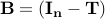Therefore, cholesky decomposition is not just an abstract mathematical manipulation but it has an intuitive interpretation in the context of modelling the time-series with autoregressive models.

Stability Selection

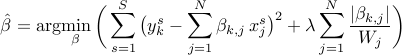
We extend this approach to randomized Lasso. The benefit is that the results are not sensitive to the parameters of the regression equations. Note that we have one parameter for each functional connection, y_k

. Randomised LASSO is a straightforward extension of LASSO and it is implemented, simply, by perturbing lambda

randomly thousands of times. The randomness is controlled by W_j

$hat{beta} = arg!min_{beta} bigg( sum_{s=1}^S big({y}^{s}_k- sum_{j=1}^N beta_{k,j},{x}^{s}_j big)^2+ lambda sum_{j=1}^N frac{|beta_{k,j}|}{W_j} bigg)$

Note that each of the extracted structural connection is associated with a probability. This probability is equal to the number of times the underlying connection was selected divided by the total number of LASSO repetitions.