4. Plotting stuff

It is sometimes said that a picture is worth a thousand words, and a quick look through any scientific journal could well convince you of this claim. Graphical representations perform a key role in science to help illustrate, explain and evaluate complex relationships.

We can produce high quality graphical representations of the functions that we are interested in using computer tools such as Wolfram Alpha, Desmos, or GeoGebra.

However, whilst we can use the computer to do plots for us, being able to idenitify various plot features without a computer is still a useful skill because the reasoning steps form the background to understanding more advanced concepts such as limits.

In this chapter we will look at the graphs of quadratics and rational fractions. After completing the chapter you should be able to plot these functions without using a computer, and identify any vertical, horizontal or oblique asymptotes.

4.1. Quadratics

The general form of a quadratic may be given in expanded form or as a completed square:

(4.1)\[\begin{align} y&=ax^2+bx+c \\ &= a\left(x+\frac{b}{2a}\right)^2+\frac{4ac-b^2}{4a} \end{align}\]

The \(y\)-intercept is at \(y=c\). The \(x\)-intercepts can be found by factorisation or use of the completed square form. The number of roots depends on the sign of the discriminant.

The shape of the plotted quadratic is called a parabola. It curves continuously in a direction that depends on the sign of \(a\), as illustrated in the schematic plots below:

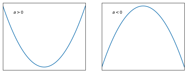
Fig. 4.1 The shape of the quadratic function \(y=ax^2+bx+c\), which is called a parabola.

The parabola has a single turning point, which can be identified from the completed square form of the quadratic function. The squared factor \(\displaystyle \left(x+\frac{b}{2a}\right)^2\) is minimised at the point

(4.2)\[\begin{equation} \biggr(x_*\ ,\ y_*\biggr)=\biggr(-\frac{b}{2a},\frac{4ac-b^2}{4a}\biggr) \end{equation}\]

• If \(a>0\) this point is a minimum

• If \(a<0\) this point is a maximum

The plot below illustrates an example case where the quadratic has two distinct real roots.

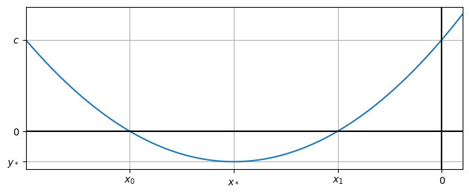
Fig. 4.2 A plot of the quadratic \(y=ax^2+bx+c\) with \(a>0\). The plot illustrates the case where there are two negative \(x_0,\ x_1\). The minimum point is denoted by \((x_* \ , \ y_*)\)

If the quadratic does not have two distinct real roots, the curve will lie entirely above or below the horizontal axis, according to the sign of \(a\). If there is a single \(x\)-intercept, this will coincide with the turning point of the function and the function will just touch the horizontal axis.

Exercise 4.1

Plot the following curves without the assistance of a computer or calculator, and without using differentiation. Describe the steps you took to deduce the shape in each case:

(a) \(y=x^2+6x+8 \qquad\) (b) \(y=x^2+6x+9 \qquad\) (c) \(y=x^2+6x+10 \qquad\)

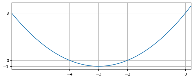
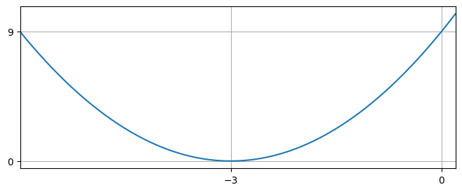
Solution to (a)

The discriminant of this quadratic is positive, so it has two real roots. The curve intercepts the \(x\) axis in two places. The roots can be found using the quadratic formula or by factorisation:

\[\begin{equation*} y=(x+4)(x+2)=0 \quad \implies \quad x=-4,-2 \end{equation*}\]

Completing the square on the quadratic gives

\[\begin{equation*} y=(x+3)^2-1 \end{equation*}\]

Therefore we can see that the minimum lies at \((-3,-1)\). This point lies midway between the two roots on the \(x\) axis, as expected owing to the symmetry of the quadratic curve. The curve intercepts the \(y\) axis at \(y=8\).

The plot of the curve therefore looks as shown below:

Solution to (b)

The discriminant of this quadratic is zero, so it has one real root, which is repeated. The curve touches the \(x\) axis in one place but does not cross it.

Completing the square on the quadratic gives

\[\begin{equation*} y=(x+3)^2 \end{equation*}\]

Therefore we can see that the single root is at the point \((-3,0)\), which is the minimum. The curve intercepts the \(y\) axis at \(y=9\).

The plot of the curve therefore looks as shown below:

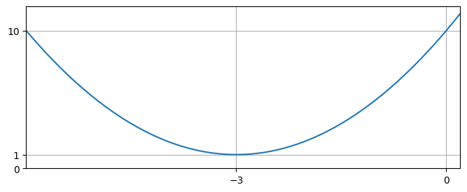
Solution to (c)

The discriminant of this quadratic is negative, so it has no real roots. The curve does not intercept the \(x\) axis.

Completing the square on the quadratic gives

\[\begin{equation*} y=(x+3)^2+1 \end{equation*}\]

Therefore we can see that the minimum is at the point \((-3,1)\). The curve intercepts the \(y\) axis at \(y=10\).

The plot of the curve therefore looks as shown below:

4.2. Reciprocals

The term reciprocal means “one over something”. The most elementary reciprocal function is

(4.3)\[\begin{equation} y=\frac{1}{x} \end{equation}\]

This fraction is undefined when \(x=0\). However, we can try some values of \(x\) that are close to zero. We observe that as \(x\) gets close to zero the fraction “blows up”, either in the positive or negative direction according to the sign of \(x\).

Demonstration

For positive values of \(x\) we obtain:

(4.4)\[\begin{align} x=\frac{1}{100} \implies y=100, \qquad \dots, \qquad x=\frac{1}{10^{10}} \implies y=10^{10}, \qquad \dots \end{align}\]

For negative values of \(x\) we obtain:

(4.5)\[\begin{align} x=\frac{-1}{100} \implies y=-100, \qquad \dots, \qquad x=\frac{-1}{10^{10}} \implies y=-10^{10}, \qquad \dots \end{align}\]

Conversely, by trying some very large values of \(x\) we observe that the fraction approaches zero, whilst remaining positive or negative according to the sign of \(x\).

Demonstration

For positive values of \(x\) we obtain:

(4.6)\[\begin{align} x=100 \implies y=\frac{1}{100}, \qquad \dots, \qquad x=10^{10} \implies y=\frac{1}{10^{10}}, \qquad \dots \end{align}\]

For negative values of \(x\) we obtain:

(4.7)\[\begin{align} x=-100 \implies y=\frac{-1}{100}, \qquad \dots, \qquad x=-10^{10} \implies y=\frac{-1}{10^{10}}, \qquad \dots \end{align}\]

We may represent these results graphically, as shown below. The dashed lines on the plot are called asymptotes. The curve continually approaches an asymptote, but does not meet it. For this function:

• The line \(y=0\) is a horizontal asymptote

• The line \(x=0\) is a vertical asymptote

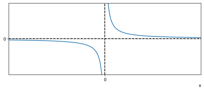
Fig. 4.3 A plot of the function \(1/x\), showing horizontal and vertical asymptotes.

We may obtain similar plots for other reciprocals.

Exercise 4.2

Identify any asymptotes of each of the following functions, and plot their curves:

(a) \(\displaystyle y=\frac{1}{x^2} \qquad\) (b) \(y=\displaystyle \frac{1}{x^2+1}\)

Solution to (a)

This function is strictly positive for all values of \(x\). It has a horizontal asymptote \(y=0\) and a vertical asymptote \(x=0\). A plot of the function is shown below:

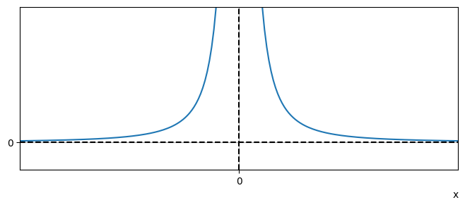
Notice that in this example the function does not change sign either side of the vertical asymptote. This is because the root \(x=0\) has multiplicity 2. A polynomial only changes sign at a root with odd-numbered multiplicity.

Solution to (b)

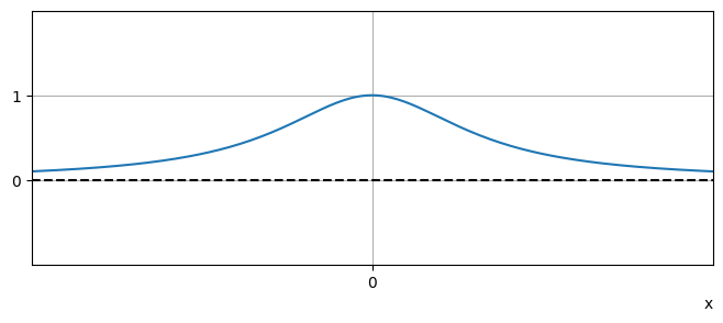
This function is strictly positive for all values of \(x\). It has a horizontal asymptote \(y=0\) but no vertical asymptote as the denominator has no roots.

The denominator is minimised when \(x=0\), and this corresponds to a maximum of \(y\). A plot of the function is shown below:

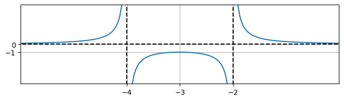
The number of vertical asymptotes is determined by the number of distinct roots of the denominator. For example, let us consider the following function:

(4.8)\[\begin{equation} y=\frac{1}{(x-2)(x-4)} \end{equation}\]

This example has a horizontal asymptote \(y=0\) and vertical asymptotes at \(x=2,4\). It is convenient to examine the sign of the function on each side of the asymptotes using a table:

	\(x<2\)	\(2<x<4\)	\(x>4\)
\((x-2)\)	-	+	+
\((x-4)\)	-	-	+
\(\displaystyle \frac{1}{(x-2)(x-4)}\)	+	-	+

By plotting the horizontal and vertical asymptotes and using the table to identify the correct sign of the function, we may deduce that \(y\) has the shape shown below:

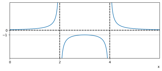
Notice that the function changes sign at each asymptote. We can anticpate this behaviour from the fact that each root has multiplicity 1.

It may not be obvious that the plot of the function should be symmetric in the line \(x=-3\). We can understand this by looking at the completed square form of the quadratic:

(4.9)\[\begin{equation} y = \frac{1}{(x-3)^2-1} \end{equation}\]

The denominator is minimised at \(x=-3\) and this corresponds to a local maximum of \(y\).

Exercise 4.3

Identify any asymptotes of each of the following functions, and plot their curves:

(a) \(\displaystyle y =\frac{1}{x^2+6x+10}\qquad\) (b) \(\displaystyle y=\frac{1}{x^2+6x+9}\qquad\) (c) \(\displaystyle y=\frac{1}{x^2+6x+8}\)

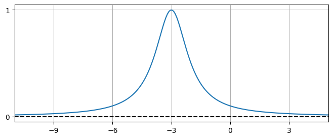
Solution to (a)

Since the discriminant of the quadratic is positive, it does not have any real roots. The denominator is strictly positive and therefore the curve lies entirely above the \(x\) axis.

Completing the square on the denominator gives

\[\begin{equation*} y=\frac{1}{(x+3)^2+1} \end{equation*}\]

The denominator is minimised when \(x=-3\) and this corresponds to the maximum of the curve. There are no vertical asymptotes, but there is a horizontal asymptote \(y=0\).

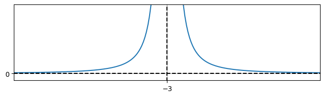
Solution to (b)

Since the discriminant of the quadratic is zero, it has one real root, which is repeated. The value of the denominator is strictly positive, except at the root. Therefore the curve lies entirely above the \(x\) axis.

Completing the square on the denominator gives

\[\begin{equation*} y=\frac{1}{(x+3)^2} \end{equation*}\]

This illustrates that there is a vertical asymptote \(x=-3\), which corresponds to a root with multiplicity 2. There is a horizontal asymptote \(y=0\).

Solution to (c)

Since the discriminant of the quadratic is positive, it has two real roots and therefore two vertical asymptotes, which are at \(x=-4,-2\).

We can examine the sign of the function in different intervals using a table:

	\(x<-4\)	\(-4<x<-2\)	\(x>-2\)
\((x+2)\)	-	-	+
\((x+4)\)	-	+	+
\(\displaystyle \frac{1}{(x+2)(x+4)}\)	+	-	+

Completing the square on the denominator gives the following result from which it can also be seen that \(x=-3\) is a local maximum:

\[\begin{equation*} y=\frac{1}{(x+3)^2-1} \end{equation*}\]

4.3. Rational fractions

We now consider the more general case of rational fractions, such as the following example. We can see that the function will have a vertical asymptote at \(x=1/2\). However, the behaviour of the function for “large” \(x\) is less obvious:

(4.10)\[y = \frac{3x^2+2x}{1-2x}\]

For these examples, we use partial fraction decomposition to make progress:

(4.11)\[\begin{equation} y= -\frac{3x}{2}-\frac{7}{4}-\frac{7}{4.(2x-1)} \end{equation}\]

The decomposition allows us to analyse what happens to the function as \(x\) becomes large, in either the positive or negative direction. In that case, the value of \(1/(2x-1)\) becomes small, and so the function approaches the oblique asymptote

\[\begin{equation*} y=-\frac{3}{2}x-\frac{7}{4} \end{equation*}\]

The sign of \(1/(2x-1)\) determines whether the function approaches the asymptote from above or below.

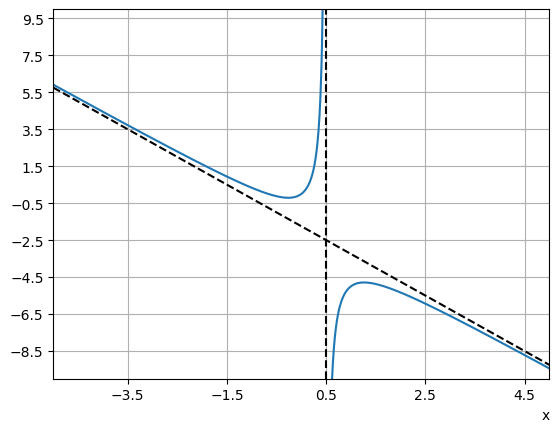
Fig. 4.4 Plotting the function \((3x^2+2x)/(1-2x)\).

Exercise 4.4

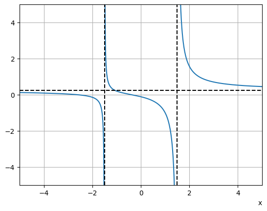
Produce a plot of the following function and identify any asymptotes:

\[\begin{equation*} y=\frac{x^2+3x+1}{(2x-3)(2x+3)} \end{equation*}\]

Solution

The function has vertical asymptotes at \(x=\pm3/2\), which each correspond to roots of multiplicity 1.

To find the other asymptotes, we use partial fraction decomposition:

\[\begin{equation*} y=\frac{1}{4}+\frac{5}{24(2x+3)}+\frac{31}{24(2x-3)} \end{equation*}\]

For large values of \(x\) the second and third terms in this decomposition shrink to zero and so the rational fraction approaches \(y=1/4\). This is a horizontal asymptote.

The plot is shown below