The easiest way to use provenance without the need to know
the syntax of the R programming language is to
start R and type the following commands at the prompt:
library(provenance)
provenance()
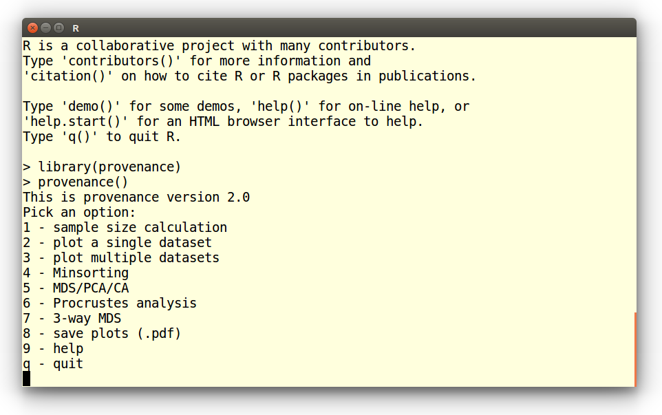
This brings up the following menu, from which the functions of
interest can be chosen:
 Tutorials:
Example 1: QFL diagrams
Example 2: Radial plots
Example 3: Kernel Density Estimates (KDEs)
Example 4: Multi-sample, multi-method summary plots
Example 5: Source Rock Density (SRD) correction
Example 6: Hydraulic sorting of heavy minerals
Example 7: Multidimensional Scaling (MDS)
Example 8: Principal Component Analysis (PCA)
Example 9: Correspondence Analysis (CA)
Example 10: 3-way MDS
Example 1: Plotting a QFL diagram
Choose option 2 from the start menu:
Pick an option:
1 - sample size calculation
2 - plot a single dataset
3 - plot multiple datasets
4 - Minsorting
5 - MDS/PCA/CA
6 - Procrustes analysis
7 - 3-way MDS
8 - save plots (.pdf)
9 - help
q - quit
2
This brings up a new list of options. Select the first of these:
Plot a single dataset:
1 - Ternary diagram
2 - Pie charts
3 - Radial plot
4 - Cumulative Age Distributions
5 - Kernel Density Estimates
1
Next you are asked to choose between two data types:
1 - Load a compositional dataset
2 - Load a point-counting dataset
The petrographic data are reported as raw counts and have not been
normalised to a common sum. So the second option is the one to choose
here. If your counting data are reported as fractions or percentages,
then you must choose the first option.
Open a compositional dataset:
Enter file name: PT.csv
This loads a petrographic dataset containing six different classes:
quartz (Q), K-feldspar (KF), plagioclase (P), and lithic fragments of
metamorphic (Lm), igneous/volcanic (Lv) and sedimentary (Ls) origin.
Next, we will amalgamate these six classes into three categories by
selecting the third option in the following list:
1 - Apply SRD correction
2 - Subset components
3 - Amalgamate components
4 - Subset samples
c - Continue
3
This brings up a nested sequence of queries, in which three new
amalgamated groups are defined: quartz (Q), feldspar (KF + P) and
lithics (Lm + Lv + Ls). The amalgamation is concluded by entering
an empty line:
Select a group of components from the following list:
Q,KF,P,Lm,Lv,Ls
Enter as a comma separated list of labels or click [Return] to exit:
Q
Name of the amalgamated component? quartz
Select a group of components from the following list:
quartz,KF,P,Lm,Lv,Ls
Enter as a comma separated list of labels or click [Return] to exit:
KF,P
Name of the amalgamated component? feldspar
Select a group of components from the following list:
feldspar,quartz,Lm,Lv,Ls
Enter as a comma separated list of labels or click [Return] to exit:
Lm,Lv,Ls
Name of the amalgamated component? lithics
Select a group of components from the following list:
lithics,feldspar,quartz
Enter as a comma separated list of labels or click [Return] to exit:
Three other functions can be combined with the amalgamation operation,
but for the sake of this tutorial, we will not use them and proceed by
entering 'c':
1 - Apply SRD correction
2 - Subset components
3 - Amalgamate components
4 - Subset samples
c - Continue
c
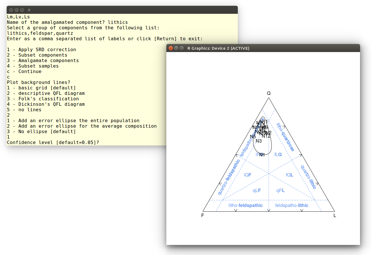
Since our amalgamated dataset contains quartz, feldspar and lithic
components, it is useful to plot it on an QFL diagram:
Plot background lines?
1 - basic grid [default]
2 - descriptive QFL diagram
3 - Folk's classification
4 - Dickinson's QFL diagram
5 - no lines
2
Finally, let's add a confidence ellipse around the data. Accept the
default value to obtain a 95% confidence region:
1 - Add an error ellipse the entire population
2 - Add an error ellipse for the average composition
3 - No ellipse [default]
1
Confidence level [default=0.05]?
This calculation may take up to a minute, because it involves the
repeated numerical solution of a double integral. Here is the
output:
Example 2: Radial plot
Point-counts are affected by a combination of (1) true compositional
variability and (2) multinomial counting uncertainties. The relative
significance of these two sources of dispersion can be visually
assessed on a radial plot. The following tutorial will use this
graphical device to assess the dispersion of the garnet-to-epidote
ratio in Namib desert sand. Select the second option from the menu:
Pick an option:
1 - sample size calculation
2 - plot a single dataset
3 - plot multiple datasets
4 - Minsorting
5 - MDS/PCA/CA
6 - Procrustes analysis
7 - 3-way MDS
8 - save plots (.pdf)
9 - help
q - quit
2
Choose the third option and open the heavy mineral dataset:
Plot a single dataset:
1 - Ternary diagram
2 - Pie charts
3 - Radial plot
4 - Cumulative Age Distributions
5 - Kernel Density Estimates
3
Open a point-counting dataset:
Enter file name: HM.csv
Accept the default options for the next step:
1 - Apply SRD correction
2 - Subset components
3 - Amalgamate components
4 - Subset samples
c - Continue
c
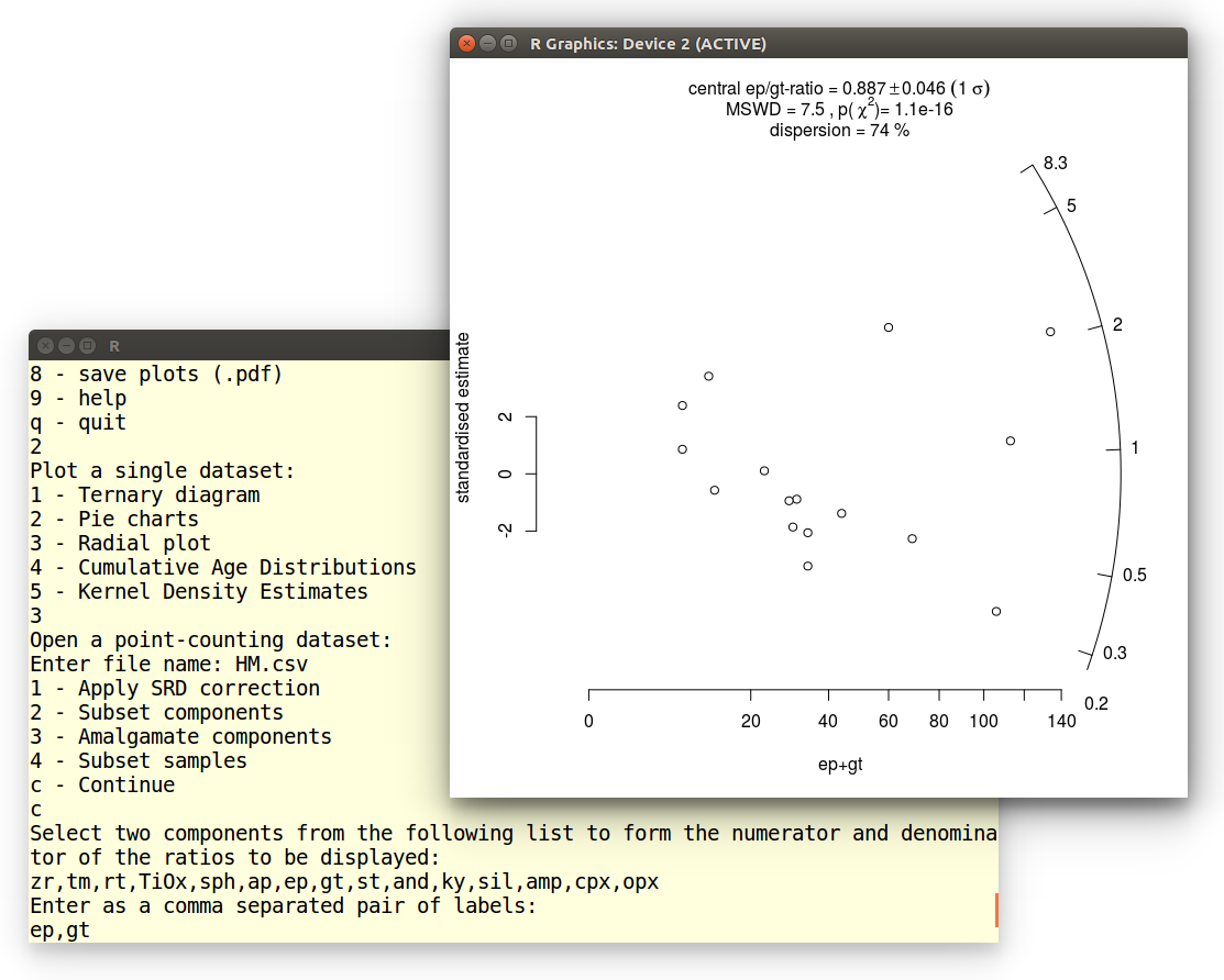
Next we are presented with all the components of HM.csv We
must choose two of these components to form a ratio. Let's select
epidote (ep) and garnet (gt):
Select two components from the following list to
form the numerator and denominator of the ratios to be displayed:
zr,tm,rt,TiOx,sph,ap,ep,gt,st,and,ky,sil,amp,cpx,opx
Enter as a comma separated pair of labels:
ep,gt
The resulting radial plot contains a lot of useful information.
First, the data scatter significantly beyond a 2-sigma error band
around the origin, indicating that the data are overdispersed with
respect to the point-counting uncertainties. This is also reflected in
the MSWD-value, which is significantly greater than 1. Equivalently,
the data fail the chi-square test for compositional homogeneity, with
a p-value of close to zero. The excess scatter of the data can be
quantified using a random effects model with 74% dispersion. This
estimates the true geological variability of the ep/gt-ratios, with
the counting uncertainties removed. Thus, the true ep/gt-ratios are
described by a lognormal distribution with a geometric mean of 0.887
± 0.046 (the 'central ratio') and a coefficient of variation
(standard deviation divided by the mean) of 0.74.
Example 3: Plot a Kernel Density Estimate (KDE)
In this tutorial we will plot a single detrital zircon U-Pb age
distribution as a KDE. After selecting the second option from the main
menu, we pick the fifth choice and open the DZ.csv datafile:
Plot a single dataset:
1 - Ternary diagram
2 - Pie charts
3 - Radial plot
4 - Cumulative Age Distributions
5 - Kernel Density Estimates
5
Open a distributional dataset:
Enter file name: DZ.csv
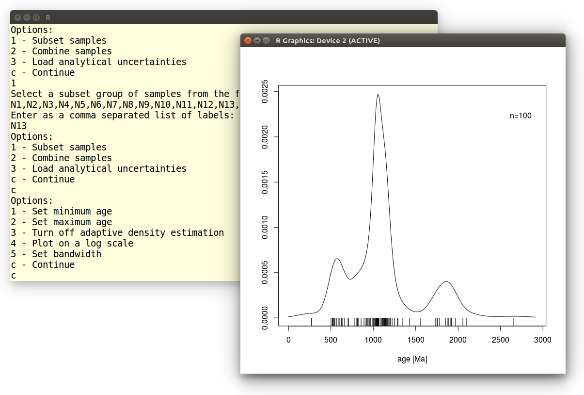
For the sake of this exercise, we will just plot a single sample
(N13), so we need to subset the multi-sample dataset. Instructions for
plotting multiple samples are given
in Example
3:
Options:
1 - Subset samples
2 - Load analytical uncertainties
c - Continue
1
Select a subset group of samples from the following list:
N1,N2,N3,N4,N5,N6,N7,N8,N9,N10,N11,N12,N13,N14,T8,T13
Enter as a comma separated list of labels:
N13
We accept the default settings for all remaining options:
Options:
1 - Subset samples
2 - Load analytical uncertainties
c - Continue
c
Options:
1 - Set minimum age
2 - Set maximum age
3 - Turn off adaptive density estimation
4 - Plot on a log scale
5 - Set bandwidth
c - Continue
c
Which produces the following graphical output:
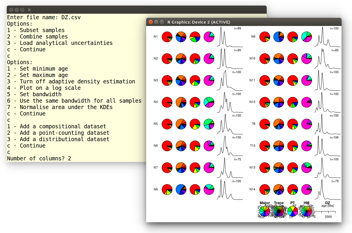
Example 4: Multi-sample, multi-method summary plot
In this tutorial, we will plot a large 15-sample, 5-method dataset
from Namibia including:
- Two compositional datasets with the Major and Trace element
compositions;
- Two point-counting datasets containing the
heavy mineral composition (HM), bulk petrography (PT);
- One distributional dataset, containing the detrital zircon
U-Pb age distributions of the same samples.
First we need to load these samples. Let's start with the major
element compositions:
1 - Add a compositional dataset
2 - Add a point-counting dataset
3 - Add a distributional dataset
c - Continue
1
Open a compositional dataset:
Enter file name: Major.csv
We get presented with a new selection menu. Let's accept the default
settings, which brings us back to the previous menu:
1 - Apply SRD correction
2 - Subset components
3 - Amalgamate components
4 - Subset samples
c - Continue
c
1 - Add a compositional dataset
2 - Add a point-counting dataset
3 - Add a distributional dataset
c - Continue
Repeat the same steps to load Trace.csv. Next, we will load
the two point-counting datasets:
1 - Add a compositional dataset
2 - Add a point-counting dataset
3 - Add a distributional dataset
c - Continue
2
Open a point-counting dataset:
Enter file name: PT.csv
1 - Apply SRD correction
2 - Subset components
3 - Amalgamate components
4 - Subset samples
c - Continue
c
Repeat for the trace element element compositions
(Trace.csv). Finally, we load the detrital zircon age
distributions:
1 - Add a compositional dataset
2 - Add a point-counting dataset
3 - Add a distributional dataset
c - Continue
3
Open a distributional dataset:
Enter file name: DZ.csv
Distributional data are plotted as Kernel Density Estimates, which can
be modified by any of seven options. For this tutorial, we will again
accept the default settings:
Options:
1 - Set minimum age
2 - Set maximum age
3 - Turn off adaptive density estimation
4 - Plot on a log scale
5 - Set bandwidth
6 - Use the same bandwidth for all samples
7 - Normalise area under the KDEs
c - Continue
c
Type 'c' again to exit the file selection menu and generate a
two-column summary plot:
1 - Add a compositional dataset
2 - Add a distributional dataset
c - Continue
c
Number of columns? 2
Which produces the following output:
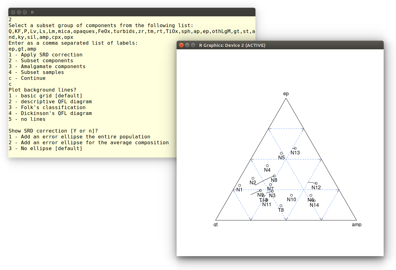
Example 5: Source Rock Density (SRD) correction
The effect of hydraulic sorting on the petrographic and heavy mineral
composition of detrital suites can be undone by restoring their
density to an assumed value. This procedure works because, a few
exceptions notwithstanding, the average density of continental crust
varies very little (between 2.65 and 2.8 g/cm3, say) over
all but the smallest catchment areas. In this tutorial, we will
visualise the SRD correction on a ternary diagram. Like in
the
first tutorial, we select the second option in the main
provenance() menu, and open a file (PTHM.csv)
containing the relative proportions of all the detrital components
(light plus heavy minerals):
Plot a single dataset:
1 - Ternary diagram
2 - Pie charts
3 - Cumulative Age Distributions
4 - Kernel Density Estimates
1
1 - Load a compositional dataset
2 - Load a point-counting dataset
1
Open a compositional dataset:
Enter file name: PTHM.csv
Note that we chose the first option because the data are expressed as
percentages and not counts. In order to apply the SRD correction, we
need to provide a table of mineral densities. provenance
comes preloaded with a set
of default
densities. We can either use these or load a different table. It
is important to make sure that the density table uses the same
category labels as the file with the sample compositions. Finally, we
need to provide the assumed density of the source rock. For this
tutorial, we will assume a 2.71 g/cm3:
1 - Apply SRD correction
2 - Subset components
3 - Amalgamate components
4 - Subset samples
c - Continue
1
Open a density file [y] or use default values [N]? n
Enter target density in g/cm3: 2.71
Since we want to plot the SRD corrected composition on a ternary
diagram, we need to reduce the number of components in the dataset
from 26 to 3. This can be done by amalgamation (see the
first
example) or subsetting, as shown next. Let's select garnet (gt),
epidote (ep) and amphibole (amp):
1 - Apply SRD correction
2 - Subset components
3 - Amalgamate components
4 - Subset samples
c - Continue
2
Select a subset group of components from the following list:
Q,KF,P,Lv,Ls,Lm,mica,opaques,FeOx,turbids,zr,tm,rt,TiOx,sph,
ap,ep,othLgM,gt,st,and,ky,sil,amp,cpx,opx
Enter as a comma separated list of labels:
ep,gt,amp
Finally, we plot the SRD-corrected gt-ep-amp composition on an empty
ternary diagram:
1 - Apply SRD correction
2 - Subset components
3 - Amalgamate components
4 - Subset samples
c - Continue
c
Plot background lines?
1 - basic grid [default]
2 - descriptive QFL diagram
3 - Folk's classification
4 - Dickinson's QFL diagram
5 - no lines
1
Show SRD correction [Y or n]? y
Where the last instruction adds lines to the diagram, showing the
effect of the SRD correction on the ep-gt-amp composition. Finally,
let's skip the error ellipse calculation:
Show SRD correction [Y or n]?
1 - Add an error ellipse the entire population
2 - Add an error ellipse for the average composition
3 - No ellipse [default]
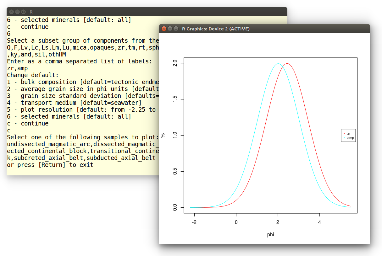
Example 6: Hydraulic sorting of heavy minerals
In this tutorial, we will compute the grain size distribution of heavy
minerals in a sediment sample. To this end, select option 4 from the
main provenance() menu. Choose the first option of the next
menu to model the heavy mineral composition of an actual sample:
Change default:
1 - bulk composition [default=tectonic endmembers]
2 - average grain size in phi units [default=2]
3 - grain size standard deviation [defaults=1]
4 - transport medium [default=seawater]
5 - plot resolution [default: from -2.25 to 5.5 by 0.05]
6 - selected minerals [default: all]
c - continue
1
1 - Load a compositional dataset
2 - Load a point-counting dataset
2
Open a point-counting dataset:
Enter file name: HM.csv
Rather than plotting all 15 minerals, select zircon (zr) and amphibole
(amp):
Change default:
1 - bulk composition [default=tectonic endmembers]
2 - average grain size in phi units [default=2]
3 - grain size standard deviation [defaults=1]
4 - transport medium [default=seawater]
5 - plot resolution [default: from -2.25 to 5.5 by 0.05]
6 - selected minerals [default: all]
c - continue
6
Select a subset group of components from the following list:
zr,tm,rt,TiOx,sph,ap,ep,gt,st,and,ky,sil,amp,cpx,opx
Enter as a comma separated list of labels:
zr,amp
Type 'c' and choose sample N1:
Change default:
1 - bulk composition [default=tectonic endmembers]
2 - average grain size in phi units [default=2]
3 - grain size standard deviation [defaults=1]
4 - transport medium [default=seawater]
5 - plot resolution [default: from -2.25 to 5.5 by 0.05]
6 - selected minerals [default: all]
c - continue
c
Select one of the following samples to plot:
N14,N13,N12,N11,N10,N9,N8,N7,N6,N5,N4,N3,N2,N1,T8,T13
or press [Return] to exit
N1
Which produces the following plot, showing that fine grained zircon is
hydraulically equivalent to coarser grained amphibole in the sample:
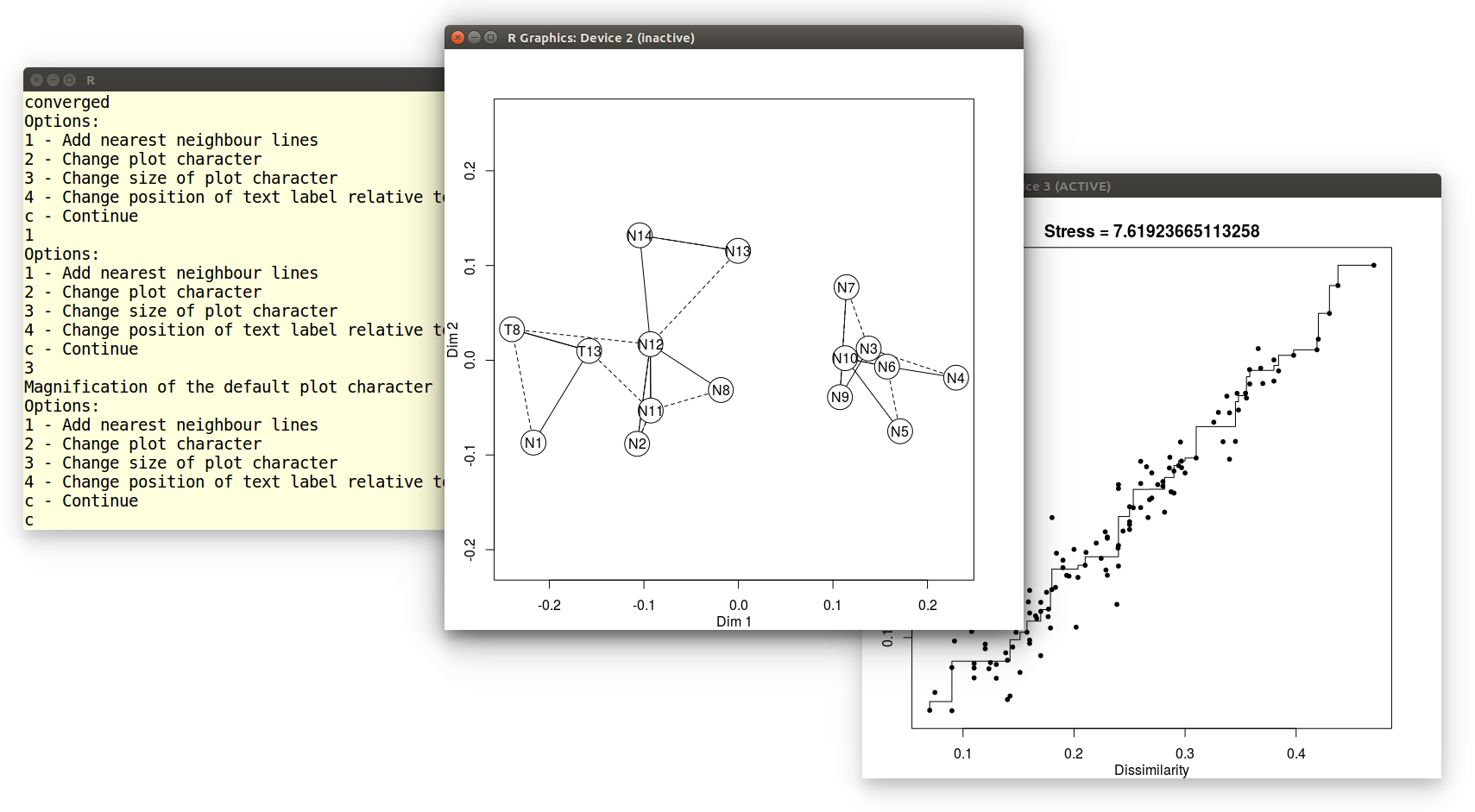
Example 7: Multidimensional Scaling (MDS)
In this tutorial we will perform an MDS analysis of the detrital
zircon dataset. After selecting the fifth option from the main menu,
we open the DZ.csv file:
1 - Load a compositional dataset
2 - Load a point-counting dataset
3 - Load a distributional dataset
3
Open a distributional dataset:
Enter file name: DZ.csv
We will use the default Kolmogorov-Smirnov dissimilarity for this
exercise. Alternatively, it is also possible to use the
Sircombe-Hazelton distance but this requires a separate input file
with analytical uncertainties. This can be done by selecting the third
option in the following menu. For this exercise, however, we will
accept the default settings:
Options:
1 - Subset samples
2 - Combine samples
3 - Load analytical uncertainties
c - Continue
c
Choose:
1 - Kolmogorov-Smirnov distance [default]
2 - Kuiper distance

initial  value 10.608343
iter   5 value 8.868203
iter   5 value 8.867183
iter  10 value 7.883745
iter  15 value 7.637849
final  value 7.619237
converged
provenance() has calculated a preliminary MDS-configuration,
using a non-metric MDS algorithm. If the stress value is extremely
low, the user is strongly encouraged to switch to classical scaling in
order to avoid overfitting the data. The stress is 7.64% in our
current example, and so the classical option is not presented
here. Finally, we can modify the visual appearance of the MDS
configuration in several ways. In this example, we will add solid
lines connecting nearest neighbours in Kolmogorov-Smirnov space (and
dashed lines connecting second-nearest neighbours), increase the size
of the plot symbols, and accept the default settings for all other
options:
Options:
1 - Add nearest neighbour lines
2 - Change plot character
3 - Change size of plot character
4 - Change position of text label relative to plot character
5 - Add X and Y axis ticks
c - Continue
1
Options:
1 - Add nearest neighbour lines
2 - Change plot character
3 - Change size of plot character
4 - Change position of text label relative to plot character
c - Continue
3
Magnification of the default plot character [1 = normal]: 4
Options:
1 - Add nearest neighbour lines
2 - Change plot character
3 - Change size of plot character
4 - Change position of text label relative to plot character
5 - Add X and Y axis ticks
c - Continue
c
This produces two pieces of graphical output: an MDS configuration and
a 'Shepard plot' illustrating the goodness of fit of the non-metric
configuration:
Example 8: Principal Component Analysis (PCA)
The previous tutorial showed how to construct an MDS configuration for
a distributional dataset. Nearly exactly the same procedure can be
applied to compositional datasets such as heavy mineral compositions
or chemical compositions. In strictly positive compositional datasets,
for which the Aitchison distance can be safely used, it is also
possible to perform Principal Component Analysis (PCA), which is a
special case of classical MDS. PCA offers the advantage that it can
jointly show the configuration and the endmember compositions as a
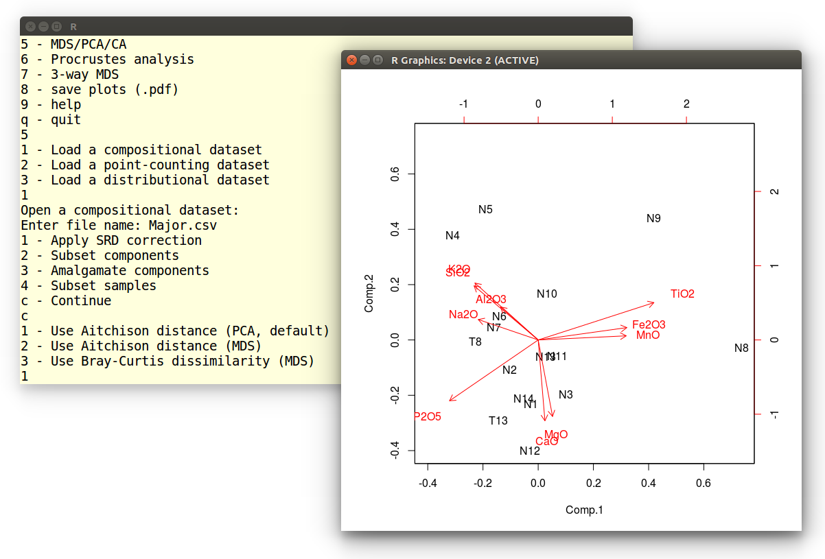
'biplot'. The current tutorial will illustrate this using the major
element composition of the Namib dataset. First, we select the fifth
option of the main provenance() menu.
Pick an option:
1 - sample size calculation
2 - plot a single dataset
3 - plot multiple datasets
4 - Minsorting
5 - MDS/PCA/CA
6 - Procrustes analysis
7 - 3-way MDS
8 - save plots (.pdf)
9 - help
q - quit
5
Next we load the Major.csv file:
1 - Load a compositional dataset
2 - Load a point-counting dataset
3 - Load a distributional dataset
1
Open a compositional dataset:
Enter file name: Major.csv
Then we accept the default settings:
1 - Apply SRD correction
2 - Subset components
3 - Amalgamate components
4 - Subset samples
c - Continue
c
At this point, we are offered three options, the first of which
performs PCA analysis:
1 - Use Aitchison distance (PCA, default)
2 - Use Aitchison distance (MDS)
3 - Use Bray-Curtis dissimilarity (MDS)
1
The resulting graphical output is shown below:
Example 9: Correspondence Analysis (CA)
To carry out a CA of point-counting data is very similar to doing
a PCA
of compositional data. We begin by choosing the fifth option of the
main menu:
Pick an option:
1 - sample size calculation
2 - plot a single dataset
3 - plot multiple datasets
4 - Minsorting
5 - MDS/PCA/CA
6 - Procrustes analysis
7 - 3-way MDS
8 - save plots (.pdf)
9 - help
q - quit
5
Load the heavy mineral compositions file as a point-counting dataset:
1 - Load a compositional dataset
2 - Load a point-counting dataset
3 - Load a distributional dataset
2
Open a point-counting dataset:
Enter file name: HM.csv
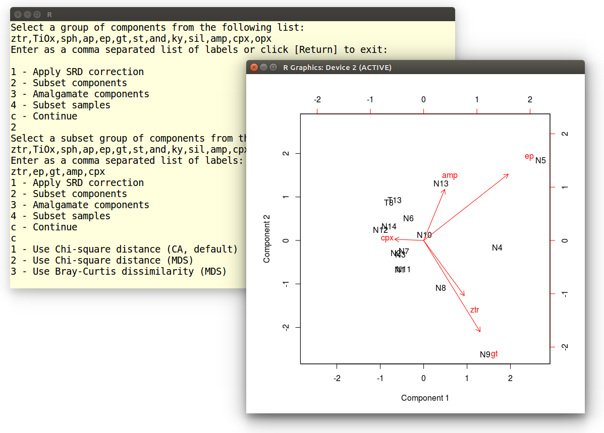
Our dataset contains 15 variables (minerals), which is a lot compared
to the 16 samples. Most of these variables are dominated by zeros.
Although CA is specifically designed to handle zeros, it is best
reduce their impact by amalgamating some components and selecting some
others. Let us begin by amalgamating the ultra-stable minerals
zircon, rutile and tourmaline.
1 - Apply SRD correction
2 - Subset components
3 - Amalgamate components
4 - Subset samples
c - Continue
3
Select a group of components from the following list:
zr,tm,rt,TiOx,sph,ap,ep,gt,st,and,ky,sil,amp,cpx,opx
Enter as a comma separated list of labels or click [Return] to exit:
zr,tm,rt
Name of the amalgamated component? ztr
We don't want to amalgamate any further components, so let's hit
[Return] to exit the amalgamation function:
Select a group of components from the following list:
ztr,TiOx,sph,ap,ep,gt,st,and,ky,sil,amp,cpx,opx
Enter as a comma separated list of labels or click [Return] to exit:
Next, we will select this newly formed ztr component with
epidote, garnet, amphibole and clinopyroxene, and discard the
remaining minerals:
1 - Apply SRD correction
2 - Subset components
3 - Amalgamate components
4 - Subset samples
c - Continue
2
Select a subset group of components from the following list:
ztr,TiOx,sph,ap,ep,gt,st,and,ky,sil,amp,cpx,opx
Enter as a comma separated list of labels:
ztr,ep,gt,amp,cpx
Enter c to continue:
1 - Apply SRD correction
2 - Subset components
3 - Amalgamate components
4 - Subset samples
c - Continue
c
Finally, select 1 (or hit [Return]) to perform the CA
and display the results as a biplot:
1 - Use Chi-square distance (CA, default)
2 - Use Chi-square distance (MDS)
3 - Use Bray-Curtis dissimilarity (MDS)
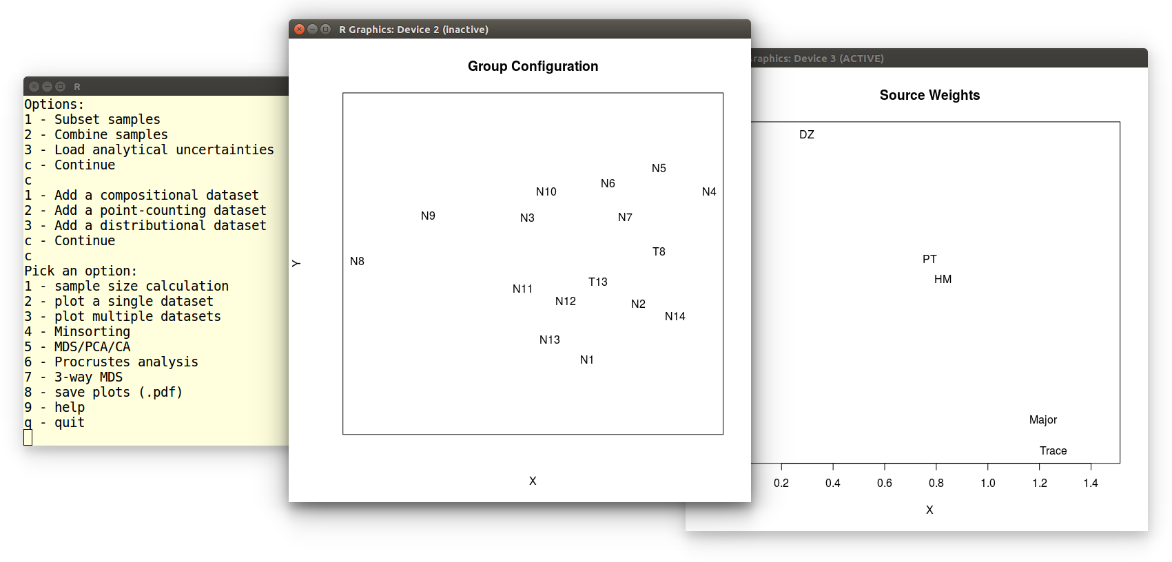
Example 10: 3-way MDS
In this tutorial, we will perform a 3-way MDS analysis of five
datasets from Namibia. After selecting the 7th option from the main
menu, loading the datasets is done as
in Example
3. The 3-way MDS function generates two pieces of graphical
output: the group configuration and subject weights:
 We can save these plots as vector-editable .pdf files by
selecting the eigth option of the main menu:
We can save these plots as vector-editable .pdf files by
selecting the eigth option of the main menu:
Pick an option:
1 - sample size calculation
2 - plot a single dataset
3 - plot multiple datasets
4 - Minsorting
5 - MDS/PCA
6 - Procrustes analysis
7 - 3-way MDS
8 - save plots (.pdf)
9 - help
q - quit
8
Enter a name for plot 2: groupconfiguration
Enter a name for plot 3: subjectweights
Which produces groupconfiguration.pdf and subjectweights.pdf.