Welcome to R!

Contents

1. Some basic R. Not (at all) exaustive.
   • These slides are designed to get you started.
   • Try this online R challenge at codeschool. Codeschool provides excellent tryouts IN YOUR BROWSER (you don’t need to install anything.
   • Have a look at many more resources about learning R on my UCL wiki
2. Some quizzes
3. Some example usage. We’ll be scratching the surface.
4. A sample applied econometric project using the FES: reading, merging, analysing, transforming data, plots and regressions
5. R and foreign Languages
6. How to make this set of slides.

Getting R and RStudio

• Click here for www.r-project.org and download R for your OS
• Click here for www.rstudio.org to download RStudio for your OS
• Take a moment to contemplate what you just did
  • you downloaded a programme from the internet without paying
  • what you did was completely legal
• As Roger Koenker would say: Buy a case of wine with what you’ve saved

Why R?

• Licensing
• Availability of add on software (packages)
• Very easy to adapt to your needs. You can look at existing code, change it and reuse it.
• Ease of connecting to other (faster) software like fortran or C
• Who uses R? (Apart from Roger Koenker?)
  • Very active and growing community in science and business.
  • data scientists use R
  • who in business uses R?

Why not R?

• steep learning curve.
• “R is slow”. Although this is a very imprecise statement. See “calling C and Fortran”.
• the sheer extent of packages available makes is hard at time to find the most suitable one
• Some people lament that the CRAN model led to a bastardization of the language, and that it should be rewritten from scratch.

Learning R if you know Matlab/Stata/other

• R for Stata Users
• R for Matlab Users
• more links on my wiki…
• get familiar with the R community. Checkout
  • Stackoverflow
  • R mailing lists on many topics

Supplementary material

• We’ll use some sample FES data and a Fortran function at some point
• if you are a git user type in your terminal

git clone git://github.com/floswald/R-demo.git

• otherwise go to https://github.com/floswald/R-demo and click on the button with the cloud and “ZIP” on it

Using this set of slides

• hit c on your keyboard for a linked table of contents. c again makes it disappear.
• left/right or mouse click or swipe takes you around
• code looks like this:

x <- 3.4
x  # print x to screen

## [1] 3.4

• the first block is input, the second block (marked with ##) is output
• everything after # is a comment
• you can (and should) type or copy and paste the code into your R and try around. All of the code you’ll see actually works.
• let’s do it.

Getting help()

• if you want help about a function, type help(fname)
• if you don’t know which function you are looking for, try `??fname``
• go to the R Site Search

Basics

• Case-sensitive: x is different from X
• fully-fledged programming language. all the usual flow controls
  • if, for, while, etc
  • check out the language definition if needed
• R needs to have all objects in memory (there are exeptions)
• R’s memory is more like matlabs and less like stata’s
  • you can have many objects of different size, type etc
  • (stata’s memory is one big spreadsheet. you can store a vector on the side, but it’s complicated.)

Assigning Values to Objects

• Everything in R (numbers, letters, vectors, functions, plots, formulas, calls,…) is an object
• assign a value (a number, a matrix, a word, a function, …) to an object with <- or = . Use <- .

x <- 3.4
x

## [1] 3.4

reassigning overwrites the current value:

x <- "now x is a character string."
x

## [1] "now x is a character string."

x <- c(3, 5, 2.1, 1001, 4.6)  # c() function combines single values into a vector.
x

## [1]    3.0    5.0    2.1 1001.0    4.6

The functions c(), str(x) and typeof(x)

• typeof(x) tells you how x was stored, mode(x) is similar
• among possible storage types are
  • logical: TRUE or FALSE
  • integer: 1, 2, 3, -10, …
  • double: 1.0, pi, -3.2331, …
  • factor: categorial variables
    • dummy vars: (0,1) labelled male,female
    • categories: (1,2,3) labelled (2,5],(5,7],(7,10]
      
  • complex: 0+0i
  • character: “hello world”
• c() requires values to have the same type (or it coerces into a common type)

typeof(x)

## [1] "double"

y <- letters[10:20]  # letters number 10 trough 20 of the english alphabet
typeof(y)

## [1] "character"

typeof(c(x, y))

## [1] "character"

str(c(x, y))  # compact display of structure of an object

##  chr [1:16] "3" "5" "2.1" "1001" "4.6" "j" "k" "l" ...

Subsetting a vector

• access the n-th element of x with x[n]
• access any tuple of elements by suppling the indices

x <- rnorm(n = 8)  # draw 8 random normal values
x

## [1]  0.4319 -0.9394 -0.2802 -0.8081  1.1112  0.1112 -0.5223 -0.6709

x[3:6]  # '3:6' produces c(3,4,5,6)

## [1] -0.2802 -0.8081  1.1112  0.1112

x[c(1, 5, 8)]  # elts 1,5 and 8

## [1]  0.4319  1.1112 -0.6709

x[-c(1, 5, 8)]  # all elts except 1,5 and 8

## [1] -0.9394 -0.2802 -0.8081  0.1112 -0.5223

Helper Functions for allocation: seq() and rep()

x <- seq(from = 1, to = 15, by = 3)  # also 'length' instead of 'by'. like matlab linspace()
x

## [1]  1  4  7 10 13

str(x)

##  num [1:5] 1 4 7 10 13

y <- rep(1:3, c(2, 3, 4))
y

## [1] 1 1 2 2 2 3 3 3 3

z <- rep(c("oh my word"), 3)
z

## [1] "oh my word" "oh my word" "oh my word"

Your turn 1

• create a vector x with values 0, 3, 6, 9, 12, 15, 18
• what is the typeof(x)?
• create a vector y containing the words {“are”,“my”,“favourite”,“numbers”}
• create a vector z from the last 2 elements of x and all of y
• what’s the typeof(z)?

Your solution 1

x <- seq(from = 0, to = 18, by = 3)
x

## [1]  0  3  6  9 12 15 18

typeof(x)

## [1] "double"

y <- c("are", "my", "favourite", "numbers")
z <- c(x[c(6, 7)], y)  # R 'coerces' x and y to a common type. here: char
z

## [1] "15"        "18"        "are"       "my"        "favourite" "numbers"

typeof(z)

## [1] "character"

Some Vector Arithmetic

• Operations +-/* are element by element

x <- 1:3
y <- 4:6
x + y

## [1] 5 7 9

• and vectors are “recycled” if they are not of the same length

x <- 1:4
x + y  # recycling the shorter vector y. R gives a warning.

## Warning: longer object length is not a multiple of shorter object length

## [1] 5 7 9 8

matrix

m1 <- matrix(data = 1:9, nrow = 3, ncol = 3, byrow = TRUE)
m2 <- matrix(data = 1:12, nrow = 4, ncol = 3, byrow = FALSE)
m1

##      [,1] [,2] [,3]
## [1,]    1    2    3
## [2,]    4    5    6
## [3,]    7    8    9

m2

##      [,1] [,2] [,3]
## [1,]    1    5    9
## [2,]    2    6   10
## [3,]    3    7   11
## [4,]    4    8   12

Combining matrices

• similarly to c() for vectors, we have cbind() and rbind()
• column-bind and row-bind

rbind(m1, m2)  # glue together the last row of of m1 and first of m2

##      [,1] [,2] [,3]
## [1,]    1    2    3
## [2,]    4    5    6
## [3,]    7    8    9
## [4,]    1    5    9
## [5,]    2    6   10
## [6,]    3    7   11
## [7,]    4    8   12

cbind(m1, t(m2))  # glue last col of m1 and first of t(m2)

##      [,1] [,2] [,3] [,4] [,5] [,6] [,7]
## [1,]    1    2    3    1    2    3    4
## [2,]    4    5    6    5    6    7    8
## [3,]    7    8    9    9   10   11   12

Subsetting a matrix

• get size of matrix with dim(m1)
• you can select indices of rows and columns. Very similar to matlab.

m1[2, ]  # row 2, all columns

## [1] 4 5 6

m2[, 1]  # all rows, column 1

## [1] 1 2 3 4

m1[c(1, 3), c(2, 3)]  # rows 1,3 and cols 2,3

##      [,1] [,2]
## [1,]    2    3
## [2,]    8    9

• or by name, if those were given:

colnames(m1) <- c("col1", "col2", "col3")
m1[, "col2"]

## [1] 2 5 8

colnames(m1) <- NULL  # remove colnames

basic matrix arithmetic

Again, +-/* are element-wise. Works only on equal sized matrices:

m1 + m2  # error

## Error: non-conformable arrays

m1 * m2  # error

## Error: non-conformable arrays

%*% is the matrix muliplication operation. matrices need to be conformable:

m2 %*% m1

##      [,1] [,2] [,3]
## [1,]   84   99  114
## [2,]   96  114  132
## [3,]  108  129  150
## [4,]  120  144  168

m1 %*% t(m2)

##      [,1] [,2] [,3] [,4]
## [1,]   38   44   50   56
## [2,]   83   98  113  128
## [3,]  128  152  176  200

m1 %*% m2

## Error: non-conformable arguments

data.frame

• A data.frame is a standard dataset
• very similar to matrix
• each row is an observation, each column is a variable
• create a data.frame from scratch with data.frame()
• Notice: all columns need to be of the same length (or recyclable)! (a data.frame is a rectangle; it’s a spreadsheet!)

df <- data.frame(cat.1 = rep(1:3, each = 2), cat.2 = 1:2, values = rnorm(6))
dim(df)

## [1] 6 3

df

##   cat.1 cat.2  values
## 1     1     1  0.8164
## 2     1     2  0.6714
## 3     2     1 -0.2564
## 4     2     2 -0.8258
## 5     3     1 -0.7887
## 6     3     2 -0.6103

Subsetting a data.frame

• A data.frame is similar to a matrix. Subsetting is thus similar.
• but additionally, you can access columns with the $ operator:

df$values

## [1]  0.8164  0.6714 -0.2564 -0.8258 -0.7887 -0.6103

• the $ in general accesses elements of “lists” (see below)
• if an element does not exist, $ adds it:

df$new.col <- df$cat.1 + df$values
df

##   cat.1 cat.2  values new.col
## 1     1     1  0.8164   1.816
## 2     1     2  0.6714   1.671
## 3     2     1 -0.2564   1.744
## 4     2     2 -0.8258   1.174
## 5     3     1 -0.7887   2.211
## 6     3     2 -0.6103   2.390

subset() 1

• get a subset of observations conditional on values of a variable

subset(df, cat.1 == 1)  # select all obs were cat.1 equals 1

##   cat.1 cat.2 values new.col
## 1     1     1 0.8164   1.816
## 2     1     2 0.6714   1.671

• this is the same as df[df$cat.1==1,]

subset() 2

• get a subset of variables

subset(df, select = c(cat.2, values))  # selects columns 'cat.2' and 'values'

##   cat.2  values
## 1     1  0.8164
## 2     2  0.6714
## 3     1 -0.2564
## 4     2 -0.8258
## 5     1 -0.7887
## 6     2 -0.6103

Removing columns

remove a column with NULL:

df$new.col <- NULL
df

##   cat.1 cat.2  values
## 1     1     1  0.8164
## 2     1     2  0.6714
## 3     2     1 -0.2564
## 4     2     2 -0.8258
## 5     3     1 -0.7887
## 6     3     2 -0.6103

Appending Data: rbind

• very similar to rbind for matrix
• If you have two data.frames with equally named columns (e.g. two editions of the same dataset), just glue together with rbind

df2 <- df  # create df2 as an exact copy of df
df2$values <- 1:nrow(df)  # but change the entries for 'values'
rbind(df, df2)  # join them row-wise

##    cat.1 cat.2  values
## 1      1     1  0.8164
## 2      1     2  0.6714
## 3      2     1 -0.2564
## 4      2     2 -0.8258
## 5      3     1 -0.7887
## 6      3     2 -0.6103
## 7      1     1  1.0000
## 8      1     2  2.0000
## 9      2     1  3.0000
## 10     2     2  4.0000
## 11     3     1  5.0000
## 12     3     2  6.0000

Looking at data.frames

• R stores datasets typically as data.frames
• special “methods”" to describe those (a method is a function that does things differently depending on the object you give it)

data(LifeCycleSavings)  # data() shows available built-in datasets
LS <- LifeCycleSavings
head(LS)  # show the first 6 rows of data.frame LifecycleSavings.

##              sr pop15 pop75    dpi ddpi
## Australia 11.43 29.35  2.87 2329.7 2.87
## Austria   12.07 23.32  4.41 1508.0 3.93
## Belgium   13.17 23.80  4.43 2108.5 3.82
## Bolivia    5.75 41.89  1.67  189.1 0.22
## Brazil    12.88 42.19  0.83  728.5 4.56
## Canada     8.79 31.72  2.85 2982.9 2.43

summary(LS)  # function summary()

##        sr            pop15          pop75           dpi      
##  Min.   : 0.60   Min.   :21.4   Min.   :0.56   Min.   :  89  
##  1st Qu.: 6.97   1st Qu.:26.2   1st Qu.:1.12   1st Qu.: 288  
##  Median :10.51   Median :32.6   Median :2.17   Median : 696  
##  Mean   : 9.67   Mean   :35.1   Mean   :2.29   Mean   :1107  
##  3rd Qu.:12.62   3rd Qu.:44.1   3rd Qu.:3.33   3rd Qu.:1796  
##  Max.   :21.10   Max.   :47.6   Max.   :4.70   Max.   :4002  
##       ddpi      
##  Min.   : 0.22  
##  1st Qu.: 2.00  
##  Median : 3.00  
##  Mean   : 3.76  
##  3rd Qu.: 4.48  
##  Max.   :16.71

ordering a data.frame

• rearrange row indices by a certain criterion
• order() and sort()
• function order(x) returns the indices of x in ascending/descending order:

order(c(5, 2, 6, 1), decreasing = TRUE)

## [1] 3 1 2 4

• plugging in a vector of indices into a matrix/data.frame, reorders the matrix according to those:

save.ranking <- order(LS$sr, decreasing = TRUE)
head(LS[save.ranking, ])

##                sr pop15 pop75    dpi ddpi
## Japan       21.10 27.01  1.91 1257.3 8.21
## Zambia      18.56 45.25  0.56  138.3 5.14
## Denmark     16.85 24.42  3.93 2496.5 3.99
## Malta       15.48 32.54  2.47  601.0 8.12
## Netherlands 14.65 24.71  3.25 1740.7 7.66
## Italy       14.28 24.52  3.48 1390.0 3.54

packages

• “packages” are add on libraries, i.e. collections of functions, algorithms and datasets
• The great number of available packages is one of the strengths of R.
• packages on CRAN have a certain degree of quality control

finding packages

• googling what you want to do often helps
• for exampe, let me google “R optimization” for you

installing packages

• install a packages available at CRAN simply by typing, for example install.packages("ggplot2")
• ggplot2 is a widely used package with plotting functions.
• load a package by calling the library function:

library(ggplot2)  # now the content of ggplot2 (functions, data, etc) are 'visible'
cut_interval  # for example, here's the code to function 'cut_interval'

## function (x, n = NULL, length = NULL, ...) 
## {
##     cut(x, breaks(x, "width", n, length), include.lowest = TRUE, 
##         ...)
## }
## <environment: namespace:ggplot2>

• get help for a package via help(package="package-name")

Functions

• R relies heavily on functions
• in fact, R is composed of functions
• look at the source code of any R function by typing the name:

matrix

## function (data = NA, nrow = 1, ncol = 1, byrow = FALSE, dimnames = NULL) 
## {
##     if (is.object(data) || !is.atomic(data)) 
##         data <- as.vector(data)
##     .Internal(matrix(data, nrow, ncol, byrow, dimnames, missing(nrow), 
##         missing(ncol)))
## }
## <bytecode: 0x100c40320>
## <environment: namespace:base>

• you can of course define your own functions.
• for example, a function to compute the interval that is “spanned” by a vector, i.e. the interval between the min and max of vector:

span <- function(x) {
    stopifnot(is.numeric(x))  # stops if x is not numeric
    r <- range(x)  # range() gives the range
    rval <- abs(r[2] - r[1])  # computes and returns the interval spanned by x
    return(rval)  # returns result
}
myvec <- rnorm(50)  # draws 50 values from the standard normal pdf
span(myvec)

## [1] 4.163

Lists

• can contain data in any “mode”: vectors, matrices, data.frames, characters, functions, plots, and more lists
• similar to a matlab or C structure

l <- list(words = c("oh my word(s)"), mats = list(mat1 = m1, mat2 = m2), 
    funs = span)
l

## $words
## [1] "oh my word(s)"
## 
## $mats
## $mats$mat1
##      [,1] [,2] [,3]
## [1,]    1    2    3
## [2,]    4    5    6
## [3,]    7    8    9
## 
## $mats$mat2
##      [,1] [,2] [,3]
## [1,]    1    5    9
## [2,]    2    6   10
## [3,]    3    7   11
## [4,]    4    8   12
## 
## 
## $funs
## function (x) 
## {
##     stopifnot(is.numeric(x))
##     r <- range(x)
##     rval <- abs(r[2] - r[1])
##     return(rval)
## }

Working with Lists

• Access a list element by position number in the list, or by name (if given)
• [["x"]] gives you element “x” as a standalone object
• ["x"] gives you element “x” as a sublist with element “x”

l[[2]]  # second list element: 'mats'

## $mat1
##      [,1] [,2] [,3]
## [1,]    1    2    3
## [2,]    4    5    6
## [3,]    7    8    9
## 
## $mat2
##      [,1] [,2] [,3]
## [1,]    1    5    9
## [2,]    2    6   10
## [3,]    3    7   11
## [4,]    4    8   12

l$mats$mat1  # of that element, the first element

##      [,1] [,2] [,3]
## [1,]    1    2    3
## [2,]    4    5    6
## [3,]    7    8    9

str(l[[1]])  # extract first element completely

##  chr "oh my word(s)"

str(l[1])  # extract first element as member of sublist

## List of 1
##  $ words: chr "oh my word(s)"

Adding and removing a new elements from a list

l$new.element <- rnorm(5)  # add a new element: 5 random draws from the standard normal
l$bool.value <- l$new.element > 0  # add a new element: previously drawn numbers positive?
l$new.element <- NULL  # delete an element
l$bool.value <- NULL
l$words <- NULL
l$funs <- NULL
l

## $mats
## $mats$mat1
##      [,1] [,2] [,3]
## [1,]    1    2    3
## [2,]    4    5    6
## [3,]    7    8    9
## 
## $mats$mat2
##      [,1] [,2] [,3]
## [1,]    1    5    9
## [2,]    2    6   10
## [3,]    3    7   11
## [4,]    4    8   12

Your Turn 2

• make a list “fruit” with two elements: “apples” and “pears”.
• for both apples and pears make up 3 pairs of random price/quantity values, e.g. for apples

observation	price	quantity
1	1.3	2
2	4.8	5
3	8.9	10

• for both apples and pears, store those values (i.e. the above table) in a data.frame with colum names “price” and “quantity”
• In other words, produce the following list. (make up your own numbers)

## $apples
##   price quantity
## 1 3.594        4
## 2 2.632        1
## 3 1.772        3
## 
## $pears
##   price quantity
## 1 1.748        1
## 2 3.635        4
## 3 2.773        2

Your Solution 2

• you can input the values by hand, for example

apples <- data.frame(price=c(1.1,2.9,1.6),quantity=c(2,3,1))

• I used the uniform random generator runif() for prices and sample() for quantities

apples <- data.frame(price = runif(min = 0, max = 4, n = 3), quantity = sample(1:4, 
    size = 3))
pears <- data.frame(price = runif(min = 0, max = 4, n = 3), quantity = sample(1:4, 
    size = 3))
fruit <- list()
fruit$apples <- apples
fruit$pears <- pears
# or all in one line:
fruit <- list(apples = data.frame(price = runif(min = 0, max = 4, 
    n = 3), quantity = sample(1:4, size = 3)), pears = data.frame(price = runif(min = 0, 
    max = 4, n = 3), quantity = sample(1:4, size = 3)))

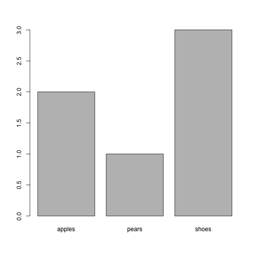
Factors

• Factors are categorical variables
• a number is given a character label
• R has plotting and tabulating methods for factors
• also nice useage in regressions

new.fac <- factor(x = c(1, 1, 2, 5, 5, 5), labels = c("apples", "pears", 
    "shoes"))
new.fac

## [1] apples apples pears  shoes  shoes  shoes 
## Levels: apples pears shoes

table(new.fac)

## new.fac
## apples  pears  shoes 
##      2      1      3

plot(new.fac)

Contingency Tables of multiple Factors

• table() can count cases of factors against each other

UCB <- as.data.frame(UCBAdmissions)  # load built-in data on Berkeley admissions
tail(UCB)  # this time, display the last 6 rows

##       Admit Gender Dept Freq
## 19 Admitted Female    E   94
## 20 Rejected Female    E  299
## 21 Admitted   Male    F   22
## 22 Rejected   Male    F  351
## 23 Admitted Female    F   24
## 24 Rejected Female    F  317

summary(UCB)  # notice how summary treats factors and numerics

##       Admit       Gender   Dept       Freq    
##  Admitted:12   Male  :12   A:4   Min.   :  8  
##  Rejected:12   Female:12   B:4   1st Qu.: 80  
##                            C:4   Median :170  
##                            D:4   Mean   :189  
##                            E:4   3rd Qu.:302  
##                            F:4   Max.   :512

table(UCB$Admit, UCB$Dept)  # table admit vs Dept?

##           
##            A B C D E F
##   Admitted 2 2 2 2 2 2
##   Rejected 2 2 2 2 2 2

• But is that what we want here?

Contingency tables 2

• No! We want to know “Freq” by those categories (those factors).
• In R-speak, what is the relationship Freq ~ factors?
• xtabs()
• takes a formula as an argument
• typical formula: y ~ x + z means “y is explained by x and z”

xtabs(Freq ~ Admit + Dept, data = UCB)  # Freq is explained by Admit and Dept

##           Dept
## Admit        A   B   C   D   E   F
##   Admitted 601 370 322 269 147  46
##   Rejected 332 215 596 523 437 668

xtabs(Freq ~ Admit + Gender, data = UCB)

##           Gender
## Admit      Male Female
##   Admitted 1198    557
##   Rejected 1493   1278

Your turn 3

• create a table that shows the number of admissions/rejections by gender AND department.

Your Solution 3

xtabs(Freq ~ Admit + Gender + Dept, data = UCB)

## , , Dept = A
## 
##           Gender
## Admit      Male Female
##   Admitted  512     89
##   Rejected  313     19
## 
## , , Dept = B
## 
##           Gender
## Admit      Male Female
##   Admitted  353     17
##   Rejected  207      8
## 
## , , Dept = C
## 
##           Gender
## Admit      Male Female
##   Admitted  120    202
##   Rejected  205    391
## 
## , , Dept = D
## 
##           Gender
## Admit      Male Female
##   Admitted  138    131
##   Rejected  279    244
## 
## , , Dept = E
## 
##           Gender
## Admit      Male Female
##   Admitted   53     94
##   Rejected  138    299
## 
## , , Dept = F
## 
##           Gender
## Admit      Male Female
##   Admitted   22     24
##   Rejected  351    317

Workspace

• In general, R needs to load an object into memory to be able to work with it
• This can be a problem with large data sets
• the function ls() shows the content of your workspace, or your current “search path”

ls()

##  [1] "%ni%"             "apples"           "df"              
##  [4] "df2"              "fruit"            "l"               
##  [7] "LifeCycleSavings" "LS"               "m1"              
## [10] "m2"               "myvec"            "new.fac"         
## [13] "pears"            "save.ranking"     "span"            
## [16] "UCB"              "x"                "y"               
## [19] "z"

rm(df, m1, m2, "%ni%", fruit, l)  # remove objects
ls()

##  [1] "apples"           "df2"              "LifeCycleSavings"
##  [4] "LS"               "myvec"            "new.fac"         
##  [7] "pears"            "save.ranking"     "span"            
## [10] "UCB"              "x"                "y"               
## [13] "z"

rm(list = ls(all = TRUE))  # remove all objects
ls()

## character(0)

A Sample Applied Econometric Project

Food and Expenditure Survey (FES)

• the repository you downloaded from github contains a folder “data”
• contains 4 files, 2 in .csv and 2 in .dta format
• each format has one data file (“fesdat”) and one file on income (“fesinc”)

Agenda

1. how to read different data
2. how to merge data
3. how to analyse data
   • with summary statistics (numerical variables)
   • in tables (categorical vars)
   • graphically
   • with statistical models
4. how to report results

R does a lot of Econometrics

• click here to get an overview of the Econometrics capabilities of R.

Reading Data Files

• Read data with with family of read.xxx() functions:
• read.csv(): comma separated values
• read.dta(): stata format
• read.table(): generic text/table reader
• library(foreign) contains many useful functions to read all sorts of foreign data formats
• library(xlsx) is useful to read .xls data

Read FES

• let’s read both .csv and .dta formats just to demonstrate:

setwd(dir = "~/git/R-demo/")  # set working directory
fesdat.csv <- read.csv(file = "data/fesdat.csv")  # read the data in csv format. Note that 'file' could also be a URL
fesinc.csv <- read.csv(file = "data/fesinc.csv")  # read the income data in csv format
library(foreign)  # load foreign to read stata data
fesdat.dta <- read.dta(file = "data/fesdat2005.dta")
fesinc.dta <- read.dta(file = "data/fesinc2005.dta")
head(fesdat.dta)  # do they look the same?

##   hhref year numads numadret numadern numhhkid kids0 kids1 kids2 kids34
## 1  2478 2005      2        0        2        0     0     0     0      0
## 2    53 2005      1        0        0        1     0     0     1      0
## 3  1085 2005      1        0        0        1     0     0     1      0
## 4  6399 2005      1        0        0        1     1     0     0      0
## 5  2441 2005      1        0        0        1     1     0     0      0
## 6  2431 2005      1        0        0        1     1     0     0      0
##   kids510 kids1116 kids1718 ncars nrooms age sex
## 1       0        0        0     1      4  17   2
## 2       0        0        0     0      5  18   2
## 3       0        0        0     0      5  18   2
## 4       0        0        0     0      5  18   2
## 5       0        0        0     0      5  18   2
## 6       0        0        0     0      4  18   2
##                                  marstat ageced educ hours foodin foodout
## 1                             cohabiting     16    0    40  38.12  15.845
## 2 Single,nev marr inc wid,div,sep pre 91      0    8     0  16.41  65.635
## 3 Single,nev marr inc wid,div,sep pre 91     16    0     0  21.39   3.300
## 4 Single,nev marr inc wid,div,sep pre 91     16    0     0  30.11   9.265
## 5 Single,nev marr inc wid,div,sep pre 91     17    0     0   8.89   5.170
## 6 Single,nev marr inc wid,div,sep pre 91     16    0     0  15.74  19.620
##     alc nondur semidur durables wfoodin wfoodout    walc   ndex lndex
## 1  8.64 171.40  11.285    11.70  0.2087  0.08673 0.04729 182.69 5.208
## 2  3.00  97.51  23.490     0.00  0.1356  0.54244 0.02479 121.00 4.796
## 3 20.00 110.33   7.500     0.00  0.1815  0.02801 0.16974 117.83 4.769
## 4  0.00  79.78   0.875     3.85  0.3733  0.11488 0.00000  80.65 4.390
## 5  0.00  34.38  26.480     2.50  0.1461  0.08495 0.00000  60.86 4.109
## 6  9.32 103.85  14.500    71.54  0.1330  0.16577 0.07875 118.35 4.774

head(fesdat.csv)

##   hhref year numads numadret numadern numhhkid kids0 kids1 kids2 kids34
## 1  2478 2005      2        0        2        0     0     0     0      0
## 2    53 2005      1        0        0        1     0     0     1      0
## 3  1085 2005      1        0        0        1     0     0     1      0
## 4  6399 2005      1        0        0        1     1     0     0      0
## 5  2441 2005      1        0        0        1     1     0     0      0
## 6  2431 2005      1        0        0        1     1     0     0      0
##   kids510 kids1116 kids1718 ncars nrooms age sex
## 1       0        0        0     1      4  17   2
## 2       0        0        0     0      5  18   2
## 3       0        0        0     0      5  18   2
## 4       0        0        0     0      5  18   2
## 5       0        0        0     0      5  18   2
## 6       0        0        0     0      4  18   2
##                                  marstat ageced educ hours foodin foodout
## 1                             cohabiting     16    0    40  38.12  15.845
## 2 Single,nev marr inc wid,div,sep pre 91      0    8     0  16.41  65.635
## 3 Single,nev marr inc wid,div,sep pre 91     16    0     0  21.39   3.300
## 4 Single,nev marr inc wid,div,sep pre 91     16    0     0  30.11   9.265
## 5 Single,nev marr inc wid,div,sep pre 91     17    0     0   8.89   5.170
## 6 Single,nev marr inc wid,div,sep pre 91     16    0     0  15.74  19.620
##     alc nondur semidur durables wfoodin wfoodout    walc   ndex lndex
## 1  8.64 171.40  11.285    11.70  0.2087  0.08673 0.04729 182.69 5.208
## 2  3.00  97.51  23.490     0.00  0.1356  0.54244 0.02479 121.00 4.796
## 3 20.00 110.33   7.500     0.00  0.1815  0.02801 0.16974 117.83 4.769
## 4  0.00  79.78   0.875     3.85  0.3733  0.11488 0.00000  80.65 4.390
## 5  0.00  34.38  26.480     2.50  0.1461  0.08495 0.00000  60.86 4.109
## 6  9.32 103.85  14.500    71.54  0.1330  0.16577 0.07875 118.35 4.774

Summary

dat <- fesdat.dta  # let's rename this to something shorter
inc <- fesinc.dta
summary(dat)

##      hhref           year          numads       numadret    
##  Min.   :   1   Min.   :2005   Min.   :1.0   Min.   :0.000  
##  1st Qu.:1697   1st Qu.:2005   1st Qu.:1.0   1st Qu.:0.000  
##  Median :3393   Median :2005   Median :2.0   Median :0.000  
##  Mean   :3393   Mean   :2005   Mean   :1.8   Mean   :0.423  
##  3rd Qu.:5089   3rd Qu.:2005   3rd Qu.:2.0   3rd Qu.:1.000  
##  Max.   :6785   Max.   :2005   Max.   :9.0   Max.   :3.000  
##                                                             
##     numadern       numhhkid         kids0            kids1       
##  Min.   :0.00   Min.   :0.000   Min.   :0.0000   Min.   :0.0000  
##  1st Qu.:0.00   1st Qu.:0.000   1st Qu.:0.0000   1st Qu.:0.0000  
##  Median :1.00   Median :0.000   Median :0.0000   Median :0.0000  
##  Mean   :1.05   Mean   :0.573   Mean   :0.0292   Mean   :0.0283  
##  3rd Qu.:2.00   3rd Qu.:1.000   3rd Qu.:0.0000   3rd Qu.:0.0000  
##  Max.   :9.00   Max.   :8.000   Max.   :2.0000   Max.   :2.0000  
##                                                                  
##      kids2            kids34         kids510         kids1116   
##  Min.   :0.0000   Min.   :0.000   Min.   :0.000   Min.   :0.00  
##  1st Qu.:0.0000   1st Qu.:0.000   1st Qu.:0.000   1st Qu.:0.00  
##  Median :0.0000   Median :0.000   Median :0.000   Median :0.00  
##  Mean   :0.0315   Mean   :0.059   Mean   :0.199   Mean   :0.19  
##  3rd Qu.:0.0000   3rd Qu.:0.000   3rd Qu.:0.000   3rd Qu.:0.00  
##  Max.   :2.0000   Max.   :5.000   Max.   :4.000   Max.   :4.00  
##                                                                 
##     kids1718          ncars          nrooms          age      
##  Min.   :0.0000   Min.   :0.00   Min.   :1.00   Min.   :17.0  
##  1st Qu.:0.0000   1st Qu.:0.00   1st Qu.:4.00   1st Qu.:38.0  
##  Median :0.0000   Median :1.00   Median :5.00   Median :51.0  
##  Mean   :0.0361   Mean   :1.08   Mean   :5.11   Mean   :51.9  
##  3rd Qu.:0.0000   3rd Qu.:2.00   3rd Qu.:6.00   3rd Qu.:66.0  
##  Max.   :2.0000   Max.   :7.00   Max.   :6.00   Max.   :80.0  
##                                                               
##       sex                                         marstat    
##  Min.   :1.00   Married spouse in household           :3349  
##  1st Qu.:1.00   Single,nev marr inc wid,div,sep pre 91:1008  
##  Median :1.00   Widowed                               : 833  
##  Mean   :1.42   Divorced                              : 722  
##  3rd Qu.:2.00   cohabiting                            : 616  
##  Max.   :2.00   Separated                             : 252  
##                 (Other)                               :   5  
##      ageced          educ           hours           foodin     
##  Min.   : 0.0   Min.   :0.000   Min.   :  0.0   Min.   :  0.0  
##  1st Qu.:15.0   1st Qu.:0.000   1st Qu.:  0.0   1st Qu.: 24.0  
##  Median :16.0   Median :0.000   Median :  0.0   Median : 40.0  
##  Mean   :16.8   Mean   :0.117   Mean   : 17.4   Mean   : 45.4  
##  3rd Qu.:18.0   3rd Qu.:0.000   3rd Qu.: 38.0   3rd Qu.: 60.9  
##  Max.   :97.0   Max.   :8.000   Max.   :104.0   Max.   :329.2  
##                                                                
##     foodout           alc            nondur         semidur     
##  Min.   :  0.0   Min.   :  0.0   Min.   :    0   Min.   :  0.0  
##  1st Qu.:  3.5   1st Qu.:  0.0   1st Qu.:  120   1st Qu.:  1.2  
##  Median : 13.0   Median :  6.0   Median :  203   Median : 15.0  
##  Mean   : 21.0   Mean   : 14.3   Mean   :  257   Mean   : 33.3  
##  3rd Qu.: 29.5   3rd Qu.: 20.0   3rd Qu.:  322   3rd Qu.: 43.0  
##  Max.   :390.2   Max.   :274.4   Max.   :10512   Max.   :811.9  
##                                                                 
##     durables         wfoodin         wfoodout           walc       
##  Min.   :-243.2   Min.   :0.000   Min.   :0.0000   Min.   :0.0000  
##  1st Qu.:   1.5   1st Qu.:0.117   1st Qu.:0.0201   1st Qu.:0.0000  
##  Median :  15.4   Median :0.184   Median :0.0565   Median :0.0250  
##  Mean   :  55.6   Mean   :0.202   Mean   :0.0701   Mean   :0.0498  
##  3rd Qu.:  60.2   3rd Qu.:0.263   3rd Qu.:0.1033   3rd Qu.:0.0715  
##  Max.   :2243.8   Max.   :0.882   Max.   :0.7741   Max.   :0.6427  
##                   NA's   :1       NA's   :1        NA's   :1       
##       ndex           lndex      
##  Min.   :    0   Min.   :0.837  
##  1st Qu.:  131   1st Qu.:4.876  
##  Median :  229   Median :5.432  
##  Mean   :  290   Mean   :5.380  
##  3rd Qu.:  368   3rd Qu.:5.908  
##  Max.   :10533   Max.   :9.262  
##                  NA's   :1

dat$year <- NULL  # we've only got one year, so useless info

Factors

str(dat$marstat)  # marstat is already a factor

##  Factor w/ 8 levels "not recorded",..: 4 5 5 5 5 5 5 5 4 4 ...

levels(dat$marstat)

## [1] "not recorded"                          
## [2] "Married spouse in household"           
## [3] "Married spouse not in household"       
## [4] "cohabiting"                            
## [5] "Single,nev marr inc wid,div,sep pre 91"
## [6] "Widowed"                               
## [7] "Divorced"                              
## [8] "Separated"

dat$sex <- factor(dat$sex, labels = c("male", "female"))  # convert sex into a factor
summary(subset(dat, select = c(sex, marstat)))

##      sex                                         marstat    
##  male  :3958   Married spouse in household           :3349  
##  female:2827   Single,nev marr inc wid,div,sep pre 91:1008  
##                Widowed                               : 833  
##                Divorced                              : 722  
##                cohabiting                            : 616  
##                Separated                             : 252  
##                (Other)                               :   5

Contingency Tables of Factors

attach(dat)  # attach(x) makes all cols of x visible on the search path
table(sex)  # otherwise I'd have to type dat$sex here

## sex
##   male female 
##   3958   2827

table(marstat, sex)

##                                         sex
## marstat                                  male female
##   not recorded                              0      0
##   Married spouse in household            2546    803
##   Married spouse not in household           4      1
##   cohabiting                              412    204
##   Single,nev marr inc wid,div,sep pre 91  474    534
##   Widowed                                 220    613
##   Divorced                                224    498
##   Separated                                78    174

More complicated tables: xtabs()

f <- ~sex + kids0
class(f)  # formula with only RHS 'explaining' variables: just get a count

## [1] "formula"

xtabs(f)

##         kids0
## sex         0    1    2
##   male   3841  115    2
##   female 2749   77    1

xtabs(~kids0 + sex + nrooms)  # three way table

## , , nrooms = 1
## 
##      sex
## kids0 male female
##     0    8      5
##     1    0      0
##     2    0      0
## 
## , , nrooms = 2
## 
##      sex
## kids0 male female
##     0   41     36
##     1    0      0
##     2    0      0
## 
## , , nrooms = 3
## 
##      sex
## kids0 male female
##     0  232    226
##     1    7      2
##     2    0      0
## 
## , , nrooms = 4
## 
##      sex
## kids0 male female
##     0  600    581
##     1   18     28
##     2    1      0
## 
## , , nrooms = 5
## 
##      sex
## kids0 male female
##     0  931    797
##     1   30     20
##     2    0      1
## 
## , , nrooms = 6
## 
##      sex
## kids0 male female
##     0 2029   1104
##     1   60     27
##     2    1      0

prop.table(xtabs(~sex + kids0), margin = 1)  # proportion of kids0 by sex

##         kids0
## sex              0         1         2
##   male   0.9704396 0.0290551 0.0005053
##   female 0.9724089 0.0272374 0.0003537

prop.table(xtabs(~sex + kids0), margin = 2)  # proportion of kids0 within age

##         kids0
## sex           0      1      2
##   male   0.5829 0.5990 0.6667
##   female 0.4171 0.4010 0.3333

detach(dat)  # remove dat from search path

Merge Data

• Both dat and inc include a unique hh identifier hhref
• use merge()

dat.inc <- merge(dat, inc, by = c("hhref"))  # if multiple keys: by=c('hhref','year')
head(dat.inc)  # note new column hhinc

##   hhref numads numadret numadern numhhkid kids0 kids1 kids2 kids34 kids510
## 1     1      1        1        0        0     0     0     0      0       0
## 2     2      2        0        2        1     0     0     0      0       0
## 3     3      1        0        0        0     0     0     0      0       0
## 4     4      2        1        1        0     0     0     0      0       0
## 5     5      3        0        3        1     0     0     0      0       0
## 6     6      1        0        1        0     0     0     0      0       0
##   kids1116 kids1718 ncars nrooms age    sex
## 1        0        0     1      6  66 female
## 2        1        0     0      4  38   male
## 3        0        0     0      3  25   male
## 4        0        0     0      3  80 female
## 5        1        0     2      6  40   male
## 6        0        0     1      4  50 female
##                                  marstat ageced educ hours foodin foodout
## 1                                Widowed     15    0     0  64.21   26.27
## 2                             cohabiting     16    0    39  75.67   10.99
## 3 Single,nev marr inc wid,div,sep pre 91      0    6     0  11.86    6.67
## 4                               Divorced     14    0     0  58.23    8.09
## 5            Married spouse in household     16    0    50  63.42   53.47
## 6                               Divorced     15    0     5  19.73    5.32
##     alc nondur semidur durables wfoodin wfoodout    walc   ndex lndex year
## 1 15.07 240.39   45.34    37.65  0.2247  0.09194 0.05274 285.73 5.655 2005
## 2 26.07 257.56   10.50    13.99  0.2823  0.04100 0.09727 268.06 5.591 2005
## 3  0.00  38.13    0.00     0.00  0.3110  0.17493 0.00000  38.13 3.641 2005
## 4 23.61 142.49  226.82    86.35  0.1577  0.02191 0.06393 369.32 5.912 2005
## 5 24.74 321.29   36.74   139.17  0.1771  0.14936 0.06910 358.02 5.881 2005
## 6 19.91  79.15    0.00     0.00  0.2492  0.06721 0.25148  79.15 4.371 2005
##    hhinc
## 1 279.95
## 2 467.07
## 3  40.00
## 4 285.46
## 5 610.95
## 6  27.18

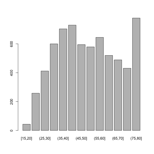
Create Bins: cut() an interval

• suppose instead of age = {17,18,19,...} we want categories of age
• base R has cut()
• ggplot2 has derived cut_interval(), bit more intuitive

dat.inc$age.cat <- cut_interval(dat.inc$age, length = 5)  # add col with age category
dat.inc$ced.cat <- cut_interval(dat.inc$ageced, length = 5)  # add col with age at educ completion category
str(dat.inc$age.cat)  # is a factor?

##  Factor w/ 13 levels "[15,20]","(20,25]",..: 11 5 2 13 5 7 3 3 3 6 ...

table(dat.inc$age.cat)

## 
## [15,20] (20,25] (25,30] (30,35] (35,40] (40,45] (45,50] (50,55] (55,60] 
##      43     258     412     600     704     730     595     579     645 
## (60,65] (65,70] (70,75] (75,80] 
##     520     489     431     779

plot(dat.inc$age.cat)

table(dat.inc$ced.cat)

## 
##    [0,5]   (5,10]  (10,15]  (15,20]  (20,25]  (25,30]  (30,35]  (35,40] 
##      103        4     2201     3471      931       55        7        0 
##  (40,45]  (45,50]  (50,55]  (55,60]  (60,65]  (65,70]  (70,75]  (75,80] 
##        1        0        0        0        0        0        0        0 
##  (80,85]  (85,90]  (90,95] (95,100] 
##        0        0        0       12

Create Bins 2: decile of income?

• Suppose we want to put people into their respective income decile

inc.dec <- quantile(dat.inc$hhinc, prob = seq(0, 1, length = 11))  # income deciles
inc.dec

##      0%     10%     20%     30%     40%     50%     60%     70%     80% 
##  -993.1   132.6   193.3   250.4   314.5   392.3   482.0   576.4   703.8 
##     90%    100% 
##   924.9 38736.5

dat.inc$inc.cat <- cut(dat.inc$hhinc, inc.dec, labels = FALSE)
head(dat.inc[, c("hhinc", "inc.cat")])  # look at columns hhinc and inc.cat

##    hhinc inc.cat
## 1 279.95       4
## 2 467.07       6
## 3  40.00       1
## 4 285.46       4
## 5 610.95       8
## 6  27.18       1

table(dat.inc$inc.cat)

## 
##   1   2   3   4   5   6   7   8   9  10 
## 678 678 679 678 679 678 678 679 678 679

Summaries by groups of Variables: library(plyr)

• Often we want summary statistics by groups of variables
• tapply(), by() and aggregate() are base R possibilities
• we’ll show library(plyr) here
• click for the amazing tutorial of plyr by Hadley Wickham
• workhorse functions are
• tranform(): transform a data.frame, (you get a df of same or bigger size)
• summarise(): summarises a data.frame (you get a df that is smaller)

summarise() and transform()

• use our FES data in dat.inc.
• functions work on an entire data.frame

library(plyr)
# summarise an entire data.frame
summarise(dat.inc, mhhinc = mean(hhinc), vhhinc = sd(hhinc), mnumads = mean(numads))

##   mhhinc vhhinc mnumads
## 1  499.2    649   1.797

# add 'income rank' to dat.inc. head(...,10) to see first 10 lines only
head(transform(dat.inc, inc.rank = rank(hhinc)), 10)

##    hhref numads numadret numadern numhhkid kids0 kids1 kids2 kids34
## 1      1      1        1        0        0     0     0     0      0
## 2      2      2        0        2        1     0     0     0      0
## 3      3      1        0        0        0     0     0     0      0
## 4      4      2        1        1        0     0     0     0      0
## 5      5      3        0        3        1     0     0     0      0
## 6      6      1        0        1        0     0     0     0      0
## 7      7      2        0        2        1     1     0     0      0
## 8      8      2        0        2        0     0     0     0      0
## 9      9      1        0        0        0     0     0     0      0
## 10    10      4        0        3        0     0     0     0      0
##    kids510 kids1116 kids1718 ncars nrooms age    sex
## 1        0        0        0     1      6  66 female
## 2        0        1        0     0      4  38   male
## 3        0        0        0     0      3  25   male
## 4        0        0        0     0      3  80 female
## 5        0        1        0     2      6  40   male
## 6        0        0        0     1      4  50 female
## 7        0        0        0     1      5  29   male
## 8        0        0        0     1      4  26 female
## 9        0        0        0     0      3  27   male
## 10       0        0        0     2      5  41 female
##                                   marstat ageced educ hours foodin foodout
## 1                                 Widowed     15    0     0  64.21   26.27
## 2                              cohabiting     16    0    39  75.67   10.99
## 3  Single,nev marr inc wid,div,sep pre 91      0    6     0  11.86    6.67
## 4                                Divorced     14    0     0  58.23    8.09
## 5             Married spouse in household     16    0    50  63.42   53.47
## 6                                Divorced     15    0     5  19.73    5.32
## 7             Married spouse in household     21    0    30  36.97    7.65
## 8                              cohabiting     17    0    38  11.64   22.36
## 9  Single,nev marr inc wid,div,sep pre 91     16    0     0  32.57   15.80
## 10            Married spouse in household     15    0     0  35.77   46.25
##       alc nondur semidur durables wfoodin wfoodout    walc   ndex lndex
## 1  15.070 240.39   45.34    37.65 0.22474  0.09194 0.05274 285.73 5.655
## 2  26.075 257.56   10.50    13.99 0.28229  0.04100 0.09727 268.06 5.591
## 3   0.000  38.13    0.00     0.00 0.31104  0.17493 0.00000  38.13 3.641
## 4  23.610 142.49  226.82    86.35 0.15767  0.02191 0.06393 369.32 5.912
## 5  24.740 321.29   36.74   139.17 0.17713  0.14936 0.06910 358.02 5.881
## 6  19.905  79.15    0.00     0.00 0.24921  0.06721 0.25148  79.15 4.371
## 7   8.235 179.33  139.79    75.14 0.11586  0.02397 0.02581 319.12 5.766
## 8  21.995 182.79    2.62    13.96 0.06275  0.12059 0.11863 185.41 5.223
## 9   0.000  64.98   14.98     0.00 0.40733  0.19760 0.00000  79.96 4.382
## 10 37.025 387.78   68.24    15.45 0.07845  0.10142 0.08119 456.02 6.123
##    year  hhinc age.cat ced.cat inc.cat inc.rank
## 1  2005 279.95 (65,70] (10,15]       4     2361
## 2  2005 467.07 (35,40] (15,20]       6     3972
## 3  2005  40.00 (20,25]   [0,5]       1       40
## 4  2005 285.46 (75,80] (10,15]       4     2419
## 5  2005 610.95 (35,40] (15,20]       8     4961
## 6  2005  27.18 (45,50] (10,15]       1       23
## 7  2005 639.37 (25,30] (20,25]       8     5109
## 8  2005 445.00 (25,30] (15,20]       6     3806
## 9  2005  91.92 (25,30] (15,20]       1      243
## 10 2005 772.30 (40,45] (10,15]       9     5679

summarise() and transform() by groups?

1. how can we get the income rank for all categories of, say, marstat?
2. can we express everybody’s income as a percentage of the highest income in each category of marstat?
3. what is the median ratio of durable to nondurable expenditure by number of rooms?
4. what is it by incoem decile?
5. what is it by both?

transform() by groups: ddply()

1. add income rank for each household for all categories of marstat to dat

head(ddply(.data = dat.inc, .variables = "marstat", .fun = transform, 
    rank.marstat = rank(hhinc)), 10)

##    hhref numads numadret numadern numhhkid kids0 kids1 kids2 kids34
## 1      5      3        0        3        1     0     0     0      0
## 2      7      2        0        2        1     1     0     0      0
## 3     10      4        0        3        0     0     0     0      0
## 4     12      2        0        1        0     0     0     0      0
## 5     13      2        0        2        2     0     0     0      0
## 6     18      2        2        0        0     0     0     0      0
## 7     20      3        0        1        0     0     0     0      0
## 8     21      2        2        0        0     0     0     0      0
## 9     24      2        0        1        0     0     0     0      0
## 10    25      2        0        1        1     0     1     0      0
##    kids510 kids1116 kids1718 ncars nrooms age    sex
## 1        0        1        0     2      6  40   male
## 2        0        0        0     1      5  29   male
## 3        0        0        0     2      5  41 female
## 4        0        0        0     1      4  50   male
## 5        0        2        0     1      5  40   male
## 6        0        0        0     1      5  73   male
## 7        0        0        0     1      6  59   male
## 8        0        0        0     0      6  73   male
## 9        0        0        0     0      5  56   male
## 10       0        0        0     1      4  22 female
##                        marstat ageced educ hours foodin foodout    alc
## 1  Married spouse in household     16    0    50  63.42   53.47 24.740
## 2  Married spouse in household     21    0    30  36.97    7.65  8.235
## 3  Married spouse in household     15    0     0  35.77   46.25 37.025
## 4  Married spouse in household     20    0     0   6.53    9.72  0.000
## 5  Married spouse in household     16    0    40  16.14   32.59 56.785
## 6  Married spouse in household     14    0     0  35.47   20.24  2.495
## 7  Married spouse in household     15    0     0 107.10   13.27 99.505
## 8  Married spouse in household     15    0     0  47.58   11.15 25.190
## 9  Married spouse in household     16    0    37  44.26    7.35 19.630
## 10 Married spouse in household     16    0     0  16.50   18.53  0.000
##    nondur semidur durables wfoodin wfoodout     walc  ndex lndex year
## 1   321.3   36.74  139.170 0.17713  0.14936 0.069102 358.0 5.881 2005
## 2   179.3  139.79   75.135 0.11586  0.02397 0.025805 319.1 5.766 2005
## 3   387.8   68.24   15.450 0.07845  0.10142 0.081193 456.0 6.123 2005
## 4   188.5   63.99   54.560 0.02586  0.03849 0.000000 252.5 5.532 2005
## 5   637.4   96.25  166.420 0.02200  0.04442 0.077396 733.7 6.598 2005
## 6   353.6   21.25   20.935 0.09462  0.05398 0.006656 374.9 5.927 2005
## 7   377.6   56.48   73.340 0.24673  0.03056 0.229237 434.1 6.073 2005
## 8   138.9   32.75    1.495 0.27723  0.06496 0.146759 171.6 5.145 2005
## 9   148.4   25.62   31.970 0.25431  0.04223 0.112777 174.1 5.159 2005
## 10  114.1    0.00    3.000 0.14470  0.16246 0.000000 114.1 4.737 2005
##    hhinc age.cat ced.cat inc.cat rank.marstat
## 1  610.9 (35,40] (15,20]       8         1991
## 2  639.4 (25,30] (20,25]       8         2097
## 3  772.3 (40,45] (10,15]       9         2490
## 4  318.7 (45,50] (15,20]       5          710
## 5  737.4 (35,40] (15,20]       9         2407
## 6  283.2 (70,75] (10,15]       4          542
## 7  395.6 (55,60] (10,15]       6         1053
## 8  297.5 (70,75] (10,15]       4          621
## 9  334.8 (55,60] (15,20]       5          776
## 10 327.6 (20,25] (15,20]       5          747

2. express everybody’s income as a percentage of the highest income in each category of marstat

head(ddply(dat.inc, "marstat", transform, perc.of.max = hhinc/max(hhinc)), 
    10)

##    hhref numads numadret numadern numhhkid kids0 kids1 kids2 kids34
## 1      5      3        0        3        1     0     0     0      0
## 2      7      2        0        2        1     1     0     0      0
## 3     10      4        0        3        0     0     0     0      0
## 4     12      2        0        1        0     0     0     0      0
## 5     13      2        0        2        2     0     0     0      0
## 6     18      2        2        0        0     0     0     0      0
## 7     20      3        0        1        0     0     0     0      0
## 8     21      2        2        0        0     0     0     0      0
## 9     24      2        0        1        0     0     0     0      0
## 10    25      2        0        1        1     0     1     0      0
##    kids510 kids1116 kids1718 ncars nrooms age    sex
## 1        0        1        0     2      6  40   male
## 2        0        0        0     1      5  29   male
## 3        0        0        0     2      5  41 female
## 4        0        0        0     1      4  50   male
## 5        0        2        0     1      5  40   male
## 6        0        0        0     1      5  73   male
## 7        0        0        0     1      6  59   male
## 8        0        0        0     0      6  73   male
## 9        0        0        0     0      5  56   male
## 10       0        0        0     1      4  22 female
##                        marstat ageced educ hours foodin foodout    alc
## 1  Married spouse in household     16    0    50  63.42   53.47 24.740
## 2  Married spouse in household     21    0    30  36.97    7.65  8.235
## 3  Married spouse in household     15    0     0  35.77   46.25 37.025
## 4  Married spouse in household     20    0     0   6.53    9.72  0.000
## 5  Married spouse in household     16    0    40  16.14   32.59 56.785
## 6  Married spouse in household     14    0     0  35.47   20.24  2.495
## 7  Married spouse in household     15    0     0 107.10   13.27 99.505
## 8  Married spouse in household     15    0     0  47.58   11.15 25.190
## 9  Married spouse in household     16    0    37  44.26    7.35 19.630
## 10 Married spouse in household     16    0     0  16.50   18.53  0.000
##    nondur semidur durables wfoodin wfoodout     walc  ndex lndex year
## 1   321.3   36.74  139.170 0.17713  0.14936 0.069102 358.0 5.881 2005
## 2   179.3  139.79   75.135 0.11586  0.02397 0.025805 319.1 5.766 2005
## 3   387.8   68.24   15.450 0.07845  0.10142 0.081193 456.0 6.123 2005
## 4   188.5   63.99   54.560 0.02586  0.03849 0.000000 252.5 5.532 2005
## 5   637.4   96.25  166.420 0.02200  0.04442 0.077396 733.7 6.598 2005
## 6   353.6   21.25   20.935 0.09462  0.05398 0.006656 374.9 5.927 2005
## 7   377.6   56.48   73.340 0.24673  0.03056 0.229237 434.1 6.073 2005
## 8   138.9   32.75    1.495 0.27723  0.06496 0.146759 171.6 5.145 2005
## 9   148.4   25.62   31.970 0.25431  0.04223 0.112777 174.1 5.159 2005
## 10  114.1    0.00    3.000 0.14470  0.16246 0.000000 114.1 4.737 2005
##    hhinc age.cat ced.cat inc.cat perc.of.max
## 1  610.9 (35,40] (15,20]       8    0.015772
## 2  639.4 (25,30] (20,25]       8    0.016506
## 3  772.3 (40,45] (10,15]       9    0.019937
## 4  318.7 (45,50] (15,20]       5    0.008226
## 5  737.4 (35,40] (15,20]       9    0.019037
## 6  283.2 (70,75] (10,15]       4    0.007311
## 7  395.6 (55,60] (10,15]       6    0.010213
## 8  297.5 (70,75] (10,15]       4    0.007681
## 9  334.8 (55,60] (15,20]       5    0.008643
## 10 327.6 (20,25] (15,20]       5    0.008458

summarise() by groups

3. median ratio of durable to nondurable expenditure by number of rooms

ddply(dat.inc, c("nrooms"), summarise, med.nondur.dur = median(nondur/durables, 
    na.rm = TRUE))

##   nrooms med.nondur.dur
## 1      1          40.98
## 2      2          26.74
## 3      3          56.71
## 4      4          17.65
## 5      5          15.02
## 6      6          10.49

4. by income decile

ddply(dat.inc, c("inc.cat"), summarise, med.nondur.dur = median(nondur/durables, 
    na.rm = T))

##    inc.cat med.nondur.dur
## 1        1         55.923
## 2        2         46.671
## 3        3         20.446
## 4        4         16.653
## 5        5         17.453
## 6        6         11.652
## 7        7         10.394
## 8        8          7.555
## 9        9          7.727
## 10      10          6.765
## 11      NA         31.173

5. by both

ddply(dat.inc, c("nrooms", "inc.cat"), summarise, med.nondur.dur = median(nondur/durables))

##    nrooms inc.cat med.nondur.dur
## 1       1       1         29.514
## 2       1       2          3.441
## 3       1       3            Inf
## 4       1       4            Inf
## 5       2       1         55.923
## 6       2       2        264.305
## 7       2       3         70.520
## 8       2       4         14.303
## 9       2       5         95.747
## 10      2       6         26.736
## 11      2       7          5.952
## 12      2       8          4.920
## 13      2       9         13.812
## 14      2      10            Inf
## 15      3       1             NA
## 16      3       2         68.800
## 17      3       3        154.473
## 18      3       4         22.531
## 19      3       5         66.409
## 20      3       6         34.023
## 21      3       7         24.682
## 22      3       8         29.883
## 23      3       9         14.360
## 24      3      10            Inf
## 25      4       1         46.028
## 26      4       2         56.398
## 27      4       3         16.572
## 28      4       4         21.661
## 29      4       5         19.852
## 30      4       6         12.512
## 31      4       7          9.620
## 32      4       8          7.562
## 33      4       9          6.118
## 34      4      10          7.868
## 35      5       1         54.167
## 36      5       2         57.002
## 37      5       3         22.446
## 38      5       4         13.884
## 39      5       5         13.223
## 40      5       6          9.310
## 41      5       7         10.243
## 42      5       8          6.880
## 43      5       9          9.338
## 44      5      10          8.861
## 45      6       1         48.133
## 46      6       2         34.481
## 47      6       3         11.674
## 48      6       4         17.718
## 49      6       5         15.791
## 50      6       6         11.948
## 51      6       7         10.505
## 52      6       8          7.740
## 53      6       9          7.374
## 54      6      10          6.549
## 55      6      NA         31.173

more ddply{plyr}

• Split data frame, apply function, and return results in a data frame.

library(plyr)
ddply(.data = dat.inc, .variables = "sex", .fun = summarise, inc = mean(hhinc))  # mean income by sex?

##      sex   inc
## 1   male 552.9
## 2 female 424.0

ddply(dat.inc, c("sex", "numads"), summarise, alc = mean(alc), foodin = mean(foodin), 
    foodout = mean(foodout))

##       sex numads     alc foodin foodout
## 1    male      1  12.335  21.64  12.512
## 2    male      2  16.085  53.34  24.060
## 3    male      3  24.062  68.01  35.314
## 4    male      4  36.492  74.62  50.590
## 5    male      5  30.686 109.28  54.595
## 6    male      6  54.084 133.02  81.595
## 7    male      7   0.000 158.16   5.625
## 8    male      8   0.000  82.87  35.075
## 9    male      9 156.450  95.94  25.695
## 10 female      1   4.710  28.72   9.080
## 11 female      2  16.455  51.37  24.505
## 12 female      3  23.975  60.93  35.894
## 13 female      4  30.336  81.28  42.586
## 14 female      5  39.619  81.89  49.511
## 15 female      6   6.657  85.10  54.789

ddply{plyr} 2

• summarise can be many things, not just mean()
• you can supply any function you want
• check out Hadley’s tutorial. ddply is very powerful.

ddply(dat.inc, "sex", summarise, age.range = median(age), car.rooms = max(ncars/nrooms))

##      sex age.range car.rooms
## 1   male        52       1.4
## 2 female        50       1.0

ddply(subset(dat.inc, numhhkid > 1), "ncars", function(x) data.frame(dur.inc = mean(x$dur/x$hhinc), 
    nondur.inc = mean(x$nondur/x$hhinc)))  # instead of summarise(), supply an 'anonymous' function

##   ncars  dur.inc nondur.inc
## 1     0 0.105007     0.6959
## 2     1 0.114872     0.6514
## 3     2 0.131991     0.6045
## 4     3 0.144138     0.6760
## 5     4 0.175777     1.5216
## 6     5 0.148054     0.5776
## 7     7 0.005687     0.6105

Alternatives to ddply

• very powerful and elegent package: data.table
• a data.table is a data.frame on speed
• excellent documentation and explainers (vignette) at CRAN
• very fast
• maybe easier to understand than ddply
• read the 10 minutes intro on the CRAN link above

summary by group with data.table

• a data.table has two indices, i and j: DT[i,j]
• i is SQL where and j is an expression

library(data.table)
dat.tab <- data.table(dat.inc)
tables()

##      NAME     NROW MB
## [1,] dat.tab 6,785 2 
##      COLS                                                                            
## [1,] hhref,numads,numadret,numadern,numhhkid,kids0,kids1,kids2,kids34,kids510,kids111
##      KEY
## [1,]    
## Total: 2MB

dat.tab[, list(median.age = as.numeric(median(age)), cars.over.rooms = median(ncars/nrooms)), 
    by = sex]

##       sex median.age cars.over.rooms
## 1: female         50          0.1667
## 2:   male         52          0.2000

# adding a column 'by reference' with :=
dat.tab[, `:=`(rel.inc, hhinc/median(hhinc))]  # I typed 'rel.inc := hhinc/median(hhinc)' here.

##       hhref numads numadret numadern numhhkid kids0 kids1 kids2 kids34
##    1:     1      1        1        0        0     0     0     0      0
##    2:     2      2        0        2        1     0     0     0      0
##    3:     3      1        0        0        0     0     0     0      0
##    4:     4      2        1        1        0     0     0     0      0
##    5:     5      3        0        3        1     0     0     0      0
##   ---                                                                 
## 6781:  6781      4        0        3        2     0     0     0      0
## 6782:  6782      2        0        1        2     0     0     0      0
## 6783:  6783      1        0        0        2     0     0     0      0
## 6784:  6784      1        1        0        0     0     0     0      0
## 6785:  6785      1        0        0        1     0     0     1      0
##       kids510 kids1116 kids1718 ncars nrooms age    sex
##    1:       0        0        0     1      6  66 female
##    2:       0        1        0     0      4  38   male
##    3:       0        0        0     0      3  25   male
##    4:       0        0        0     0      3  80 female
##    5:       0        1        0     2      6  40   male
##   ---                                                  
## 6781:       0        1        1     3      6  42   male
## 6782:       0        1        1     1      6  49   male
## 6783:       0        2        0     1      5  33 female
## 6784:       0        0        0     0      5  76 female
## 6785:       0        0        0     0      5  24 female
##                                      marstat ageced educ hours foodin
##    1:                                Widowed     15    0     0  64.21
##    2:                             cohabiting     16    0    39  75.67
##    3: Single,nev marr inc wid,div,sep pre 91      0    6     0  11.86
##    4:                               Divorced     14    0     0  58.23
##    5:            Married spouse in household     16    0    50  63.42
##   ---                                                                
## 6781:            Married spouse in household     16    0     0 122.00
## 6782:            Married spouse in household     16    0     0  22.48
## 6783:                               Divorced     18    0     0  18.45
## 6784:                                Widowed     15    0     0  35.31
## 6785: Single,nev marr inc wid,div,sep pre 91     16    0     0   0.00
##       foodout    alc nondur semidur durables wfoodin wfoodout    walc
##    1:   26.27  15.07 240.39   45.34   37.650 0.22474  0.09194 0.05274
##    2:   10.99  26.07 257.56   10.50   13.995 0.28229  0.04100 0.09727
##    3:    6.67   0.00  38.13    0.00    0.000 0.31104  0.17493 0.00000
##    4:    8.09  23.61 142.49  226.82   86.355 0.15767  0.02191 0.06393
##    5:   53.47  24.74 321.29   36.74  139.170 0.17713  0.14936 0.06910
##   ---                                                                
## 6781:   50.25 120.50 641.52   64.52   98.320 0.17280  0.07117 0.17067
## 6782:   88.90  31.35 393.19   71.12    9.620 0.04840  0.19147 0.06751
## 6783:    5.90   0.00 206.65   67.00    6.995 0.06744  0.02156 0.00000
## 6784:    0.00   0.00  95.53    0.00    1.255 0.36964  0.00000 0.00000
## 6785:    0.00   0.00  97.00    0.00  165.000 0.00000  0.00000 0.00000
##         ndex lndex year  hhinc age.cat ced.cat inc.cat rel.inc
##    1: 285.73 5.655 2005  280.0 (65,70] (10,15]       4  0.7136
##    2: 268.06 5.591 2005  467.1 (35,40] (15,20]       6  1.1905
##    3:  38.13 3.641 2005   40.0 (20,25]   [0,5]       1  0.1020
##    4: 369.32 5.912 2005  285.5 (75,80] (10,15]       4  0.7276
##    5: 358.02 5.881 2005  610.9 (35,40] (15,20]       8  1.5572
##   ---                                                         
## 6781: 706.04 6.560 2005 1184.2 (40,45] (15,20]      10  3.0185
## 6782: 464.31 6.141 2005  388.2 (45,50] (15,20]       5  0.9896
## 6783: 273.65 5.612 2005  248.6 (30,35] (15,20]       3  0.6337
## 6784:  95.53 4.559 2005  113.5 (75,80] (10,15]       1  0.2893
## 6785:  97.00 4.575 2005  120.0 (20,25] (15,20]       1  0.3059

dat.tab[, `:=`(rel.inc.sex, hhinc/median(hhinc)), by = sex]

##       hhref numads numadret numadern numhhkid kids0 kids1 kids2 kids34
##    1:     1      1        1        0        0     0     0     0      0
##    2:     2      2        0        2        1     0     0     0      0
##    3:     3      1        0        0        0     0     0     0      0
##    4:     4      2        1        1        0     0     0     0      0
##    5:     5      3        0        3        1     0     0     0      0
##   ---                                                                 
## 6781:  6781      4        0        3        2     0     0     0      0
## 6782:  6782      2        0        1        2     0     0     0      0
## 6783:  6783      1        0        0        2     0     0     0      0
## 6784:  6784      1        1        0        0     0     0     0      0
## 6785:  6785      1        0        0        1     0     0     1      0
##       kids510 kids1116 kids1718 ncars nrooms age    sex
##    1:       0        0        0     1      6  66 female
##    2:       0        1        0     0      4  38   male
##    3:       0        0        0     0      3  25   male
##    4:       0        0        0     0      3  80 female
##    5:       0        1        0     2      6  40   male
##   ---                                                  
## 6781:       0        1        1     3      6  42   male
## 6782:       0        1        1     1      6  49   male
## 6783:       0        2        0     1      5  33 female
## 6784:       0        0        0     0      5  76 female
## 6785:       0        0        0     0      5  24 female
##                                      marstat ageced educ hours foodin
##    1:                                Widowed     15    0     0  64.21
##    2:                             cohabiting     16    0    39  75.67
##    3: Single,nev marr inc wid,div,sep pre 91      0    6     0  11.86
##    4:                               Divorced     14    0     0  58.23
##    5:            Married spouse in household     16    0    50  63.42
##   ---                                                                
## 6781:            Married spouse in household     16    0     0 122.00
## 6782:            Married spouse in household     16    0     0  22.48
## 6783:                               Divorced     18    0     0  18.45
## 6784:                                Widowed     15    0     0  35.31
## 6785: Single,nev marr inc wid,div,sep pre 91     16    0     0   0.00
##       foodout    alc nondur semidur durables wfoodin wfoodout    walc
##    1:   26.27  15.07 240.39   45.34   37.650 0.22474  0.09194 0.05274
##    2:   10.99  26.07 257.56   10.50   13.995 0.28229  0.04100 0.09727
##    3:    6.67   0.00  38.13    0.00    0.000 0.31104  0.17493 0.00000
##    4:    8.09  23.61 142.49  226.82   86.355 0.15767  0.02191 0.06393
##    5:   53.47  24.74 321.29   36.74  139.170 0.17713  0.14936 0.06910
##   ---                                                                
## 6781:   50.25 120.50 641.52   64.52   98.320 0.17280  0.07117 0.17067
## 6782:   88.90  31.35 393.19   71.12    9.620 0.04840  0.19147 0.06751
## 6783:    5.90   0.00 206.65   67.00    6.995 0.06744  0.02156 0.00000
## 6784:    0.00   0.00  95.53    0.00    1.255 0.36964  0.00000 0.00000
## 6785:    0.00   0.00  97.00    0.00  165.000 0.00000  0.00000 0.00000
##         ndex lndex year  hhinc age.cat ced.cat inc.cat rel.inc rel.inc.sex
##    1: 285.73 5.655 2005  280.0 (65,70] (10,15]       4  0.7136     0.92498
##    2: 268.06 5.591 2005  467.1 (35,40] (15,20]       6  1.1905     1.01540
##    3:  38.13 3.641 2005   40.0 (20,25]   [0,5]       1  0.1020     0.08696
##    4: 369.32 5.912 2005  285.5 (75,80] (10,15]       4  0.7276     0.94320
##    5: 358.02 5.881 2005  610.9 (35,40] (15,20]       8  1.5572     1.32818
##   ---                                                                     
## 6781: 706.04 6.560 2005 1184.2 (40,45] (15,20]      10  3.0185     2.57446
## 6782: 464.31 6.141 2005  388.2 (45,50] (15,20]       5  0.9896     0.84404
## 6783: 273.65 5.612 2005  248.6 (30,35] (15,20]       3  0.6337     0.82140
## 6784:  95.53 4.559 2005  113.5 (75,80] (10,15]       1  0.2893     0.37499
## 6785:  97.00 4.575 2005  120.0 (20,25] (15,20]       1  0.3059     0.39649

dat.tab[, `:=`(rel.inc.sex.nrooms, hhinc/median(hhinc)), by = list(sex, 
    nrooms)]

##       hhref numads numadret numadern numhhkid kids0 kids1 kids2 kids34
##    1:     1      1        1        0        0     0     0     0      0
##    2:     2      2        0        2        1     0     0     0      0
##    3:     3      1        0        0        0     0     0     0      0
##    4:     4      2        1        1        0     0     0     0      0
##    5:     5      3        0        3        1     0     0     0      0
##   ---                                                                 
## 6781:  6781      4        0        3        2     0     0     0      0
## 6782:  6782      2        0        1        2     0     0     0      0
## 6783:  6783      1        0        0        2     0     0     0      0
## 6784:  6784      1        1        0        0     0     0     0      0
## 6785:  6785      1        0        0        1     0     0     1      0
##       kids510 kids1116 kids1718 ncars nrooms age    sex
##    1:       0        0        0     1      6  66 female
##    2:       0        1        0     0      4  38   male
##    3:       0        0        0     0      3  25   male
##    4:       0        0        0     0      3  80 female
##    5:       0        1        0     2      6  40   male
##   ---                                                  
## 6781:       0        1        1     3      6  42   male
## 6782:       0        1        1     1      6  49   male
## 6783:       0        2        0     1      5  33 female
## 6784:       0        0        0     0      5  76 female
## 6785:       0        0        0     0      5  24 female
##                                      marstat ageced educ hours foodin
##    1:                                Widowed     15    0     0  64.21
##    2:                             cohabiting     16    0    39  75.67
##    3: Single,nev marr inc wid,div,sep pre 91      0    6     0  11.86
##    4:                               Divorced     14    0     0  58.23
##    5:            Married spouse in household     16    0    50  63.42
##   ---                                                                
## 6781:            Married spouse in household     16    0     0 122.00
## 6782:            Married spouse in household     16    0     0  22.48
## 6783:                               Divorced     18    0     0  18.45
## 6784:                                Widowed     15    0     0  35.31
## 6785: Single,nev marr inc wid,div,sep pre 91     16    0     0   0.00
##       foodout    alc nondur semidur durables wfoodin wfoodout    walc
##    1:   26.27  15.07 240.39   45.34   37.650 0.22474  0.09194 0.05274
##    2:   10.99  26.07 257.56   10.50   13.995 0.28229  0.04100 0.09727
##    3:    6.67   0.00  38.13    0.00    0.000 0.31104  0.17493 0.00000
##    4:    8.09  23.61 142.49  226.82   86.355 0.15767  0.02191 0.06393
##    5:   53.47  24.74 321.29   36.74  139.170 0.17713  0.14936 0.06910
##   ---                                                                
## 6781:   50.25 120.50 641.52   64.52   98.320 0.17280  0.07117 0.17067
## 6782:   88.90  31.35 393.19   71.12    9.620 0.04840  0.19147 0.06751
## 6783:    5.90   0.00 206.65   67.00    6.995 0.06744  0.02156 0.00000
## 6784:    0.00   0.00  95.53    0.00    1.255 0.36964  0.00000 0.00000
## 6785:    0.00   0.00  97.00    0.00  165.000 0.00000  0.00000 0.00000
##         ndex lndex year  hhinc age.cat ced.cat inc.cat rel.inc rel.inc.sex
##    1: 285.73 5.655 2005  280.0 (65,70] (10,15]       4  0.7136     0.92498
##    2: 268.06 5.591 2005  467.1 (35,40] (15,20]       6  1.1905     1.01540
##    3:  38.13 3.641 2005   40.0 (20,25]   [0,5]       1  0.1020     0.08696
##    4: 369.32 5.912 2005  285.5 (75,80] (10,15]       4  0.7276     0.94320
##    5: 358.02 5.881 2005  610.9 (35,40] (15,20]       8  1.5572     1.32818
##   ---                                                                     
## 6781: 706.04 6.560 2005 1184.2 (40,45] (15,20]      10  3.0185     2.57446
## 6782: 464.31 6.141 2005  388.2 (45,50] (15,20]       5  0.9896     0.84404
## 6783: 273.65 5.612 2005  248.6 (30,35] (15,20]       3  0.6337     0.82140
## 6784:  95.53 4.559 2005  113.5 (75,80] (10,15]       1  0.2893     0.37499
## 6785:  97.00 4.575 2005  120.0 (20,25] (15,20]       1  0.3059     0.39649
##       rel.inc.sex.nrooms
##    1:             0.6235
##    2:             1.4289
##    3:             0.1760
##    4:             1.6725
##    5:             1.0829
##   ---                   
## 6781:             2.0990
## 6782:             0.6882
## 6783:             0.9589
## 6784:             0.4378
## 6785:             0.4629

data.tables and keys

• very large speed gain by avoiding vector scan and using binary search instead
• you set a key on a table, like a database

setkey(dat.tab, numhhkid)
dat.tab[numhhkid == 1]

##      hhref numads numadret numadern numhhkid kids0 kids1 kids2 kids34
##   1:     2      2        0        2        1     0     0     0      0
##   2:     5      3        0        3        1     0     0     0      0
##   3:     7      2        0        2        1     1     0     0      0
##   4:    17      2        0        0        1     0     0     0      1
##   5:    25      2        0        1        1     0     1     0      0
##  ---                                                                 
## 898:  6751      2        0        2        1     0     0     0      0
## 899:  6765      2        0        1        1     0     0     0      1
## 900:  6776      2        0        1        1     0     0     0      1
## 901:  6777      2        0        2        1     0     0     0      0
## 902:  6785      1        0        0        1     0     0     1      0
##      kids510 kids1116 kids1718 ncars nrooms age    sex
##   1:       0        1        0     0      4  38   male
##   2:       0        1        0     2      6  40   male
##   3:       0        0        0     1      5  29   male
##   4:       0        0        0     0      5  22 female
##   5:       0        0        0     1      4  22 female
##  ---                                                  
## 898:       1        0        0     2      6  57   male
## 899:       0        0        0     1      6  33   male
## 900:       0        0        0     1      6  25   male
## 901:       0        1        0     2      6  47   male
## 902:       0        0        0     0      5  24 female
##                                     marstat ageced educ hours foodin
##   1:                             cohabiting     16    0    39  75.67
##   2:            Married spouse in household     16    0    50  63.42
##   3:            Married spouse in household     21    0    30  36.97
##   4:                             cohabiting     16    0     0  10.33
##   5:            Married spouse in household     16    0     0  16.50
##  ---                                                                
## 898:            Married spouse in household     21    0    40 148.51
## 899:                             cohabiting     19    0     0  46.60
## 900:            Married spouse in household     18    0    38  35.83
## 901:            Married spouse in household     21    0    37 100.82
## 902: Single,nev marr inc wid,div,sep pre 91     16    0     0   0.00
##      foodout    alc nondur semidur durables wfoodin wfoodout     walc
##   1:   10.99 26.075 257.56   10.50    13.99  0.2823  0.04100 0.097274
##   2:   53.47 24.740 321.29   36.74   139.17  0.1771  0.14936 0.069102
##   3:    7.65  8.235 179.33  139.79    75.14  0.1159  0.02397 0.025805
##   4:    5.37  0.000  48.88    8.00     0.00  0.1816  0.09440 0.000000
##   5:   18.53  0.000 114.06    0.00     3.00  0.1447  0.16246 0.000000
##  ---                                                                 
## 898:   47.80  2.590 633.84   56.62     0.58  0.2151  0.06923 0.003751
## 899:   33.55 36.765 288.63   77.24   107.65  0.1274  0.09170 0.100487
## 900:   72.55 29.500 248.35   89.00     9.69  0.1062  0.21506 0.087448
## 901:   56.49  0.000 735.15  136.02    70.88  0.1157  0.06485 0.000000
## 902:    0.00  0.000  97.00    0.00   165.00  0.0000  0.00000 0.000000
##        ndex lndex year  hhinc age.cat ced.cat inc.cat rel.inc rel.inc.sex
##   1: 268.06 5.591 2005  467.1 (35,40] (15,20]       6  1.1905      1.0154
##   2: 358.02 5.881 2005  610.9 (35,40] (15,20]       8  1.5572      1.3282
##   3: 319.12 5.766 2005  639.4 (25,30] (20,25]       8  1.6297      1.3900
##   4:  56.88 4.041 2005  182.2 (20,25] (15,20]       2  0.4645      0.6021
##   5: 114.06 4.737 2005  327.6 (20,25] (15,20]       5  0.8351      1.0826
##  ---                                                                     
## 898: 690.46 6.537 2005 1192.1 (55,60] (20,25]      10  3.0385      2.5915
## 899: 365.87 5.902 2005  405.8 (30,35] (15,20]       6  1.0344      0.8823
## 900: 337.35 5.821 2005  321.6 (20,25] (15,20]       5  0.8198      0.6992
## 901: 871.17 6.770 2005  903.6 (45,50] (20,25]       9  2.3032      1.9644
## 902:  97.00 4.575 2005  120.0 (20,25] (15,20]       1  0.3059      0.3965
##      rel.inc.sex.nrooms
##   1:             1.4289
##   2:             1.0829
##   3:             1.5904
##   4:             0.7028
##   5:             1.4260
##  ---                   
## 898:             2.1129
## 899:             0.7193
## 900:             0.5701
## 901:             1.6016
## 902:             0.4629

dat.tab[J(1)]

##      numhhkid hhref numads numadret numadern kids0 kids1 kids2 kids34
##   1:        1     2      2        0        2     0     0     0      0
##   2:        1     5      3        0        3     0     0     0      0
##   3:        1     7      2        0        2     1     0     0      0
##   4:        1    17      2        0        0     0     0     0      1
##   5:        1    25      2        0        1     0     1     0      0
##  ---                                                                 
## 898:        1  6751      2        0        2     0     0     0      0
## 899:        1  6765      2        0        1     0     0     0      1
## 900:        1  6776      2        0        1     0     0     0      1
## 901:        1  6777      2        0        2     0     0     0      0
## 902:        1  6785      1        0        0     0     0     1      0
##      kids510 kids1116 kids1718 ncars nrooms age    sex
##   1:       0        1        0     0      4  38   male
##   2:       0        1        0     2      6  40   male
##   3:       0        0        0     1      5  29   male
##   4:       0        0        0     0      5  22 female
##   5:       0        0        0     1      4  22 female
##  ---                                                  
## 898:       1        0        0     2      6  57   male
## 899:       0        0        0     1      6  33   male
## 900:       0        0        0     1      6  25   male
## 901:       0        1        0     2      6  47   male
## 902:       0        0        0     0      5  24 female
##                                     marstat ageced educ hours foodin
##   1:                             cohabiting     16    0    39  75.67
##   2:            Married spouse in household     16    0    50  63.42
##   3:            Married spouse in household     21    0    30  36.97
##   4:                             cohabiting     16    0     0  10.33
##   5:            Married spouse in household     16    0     0  16.50
##  ---                                                                
## 898:            Married spouse in household     21    0    40 148.51
## 899:                             cohabiting     19    0     0  46.60
## 900:            Married spouse in household     18    0    38  35.83
## 901:            Married spouse in household     21    0    37 100.82
## 902: Single,nev marr inc wid,div,sep pre 91     16    0     0   0.00
##      foodout    alc nondur semidur durables wfoodin wfoodout     walc
##   1:   10.99 26.075 257.56   10.50    13.99  0.2823  0.04100 0.097274
##   2:   53.47 24.740 321.29   36.74   139.17  0.1771  0.14936 0.069102
##   3:    7.65  8.235 179.33  139.79    75.14  0.1159  0.02397 0.025805
##   4:    5.37  0.000  48.88    8.00     0.00  0.1816  0.09440 0.000000
##   5:   18.53  0.000 114.06    0.00     3.00  0.1447  0.16246 0.000000
##  ---                                                                 
## 898:   47.80  2.590 633.84   56.62     0.58  0.2151  0.06923 0.003751
## 899:   33.55 36.765 288.63   77.24   107.65  0.1274  0.09170 0.100487
## 900:   72.55 29.500 248.35   89.00     9.69  0.1062  0.21506 0.087448
## 901:   56.49  0.000 735.15  136.02    70.88  0.1157  0.06485 0.000000
## 902:    0.00  0.000  97.00    0.00   165.00  0.0000  0.00000 0.000000
##        ndex lndex year  hhinc age.cat ced.cat inc.cat rel.inc rel.inc.sex
##   1: 268.06 5.591 2005  467.1 (35,40] (15,20]       6  1.1905      1.0154
##   2: 358.02 5.881 2005  610.9 (35,40] (15,20]       8  1.5572      1.3282
##   3: 319.12 5.766 2005  639.4 (25,30] (20,25]       8  1.6297      1.3900
##   4:  56.88 4.041 2005  182.2 (20,25] (15,20]       2  0.4645      0.6021
##   5: 114.06 4.737 2005  327.6 (20,25] (15,20]       5  0.8351      1.0826
##  ---                                                                     
## 898: 690.46 6.537 2005 1192.1 (55,60] (20,25]      10  3.0385      2.5915
## 899: 365.87 5.902 2005  405.8 (30,35] (15,20]       6  1.0344      0.8823
## 900: 337.35 5.821 2005  321.6 (20,25] (15,20]       5  0.8198      0.6992
## 901: 871.17 6.770 2005  903.6 (45,50] (20,25]       9  2.3032      1.9644
## 902:  97.00 4.575 2005  120.0 (20,25] (15,20]       1  0.3059      0.3965
##      rel.inc.sex.nrooms
##   1:             1.4289
##   2:             1.0829
##   3:             1.5904
##   4:             0.7028
##   5:             1.4260
##  ---                   
## 898:             2.1129
## 899:             0.7193
## 900:             0.5701
## 901:             1.6016
## 902:             0.4629

dat.tab[J(2), `:=`(twokid.foodin, log(foodin)/log(foodout))]

##       hhref numads numadret numadern numhhkid kids0 kids1 kids2 kids34
##    1:     1      1        1        0        0     0     0     0      0
##    2:     3      1        0        0        0     0     0     0      0
##    3:     4      2        1        1        0     0     0     0      0
##    4:     6      1        0        1        0     0     0     0      0
##    5:     8      2        0        2        0     0     0     0      0
##   ---                                                                 
## 6781:  3230      3        0        2        7     0     1     0      1
## 6782:  3466      6        0        0        7     0     0     1      5
## 6783:  4824      4        0        3        7     0     0     0      2
## 6784:  6629      2        0        1        7     0     0     0      1
## 6785:  4787      1        0        1        8     1     0     2      0
##       kids510 kids1116 kids1718 ncars nrooms age    sex
##    1:       0        0        0     1      6  66 female
##    2:       0        0        0     0      3  25   male
##    3:       0        0        0     0      3  80 female
##    4:       0        0        0     1      4  50 female
##    5:       0        0        0     1      4  26 female
##   ---                                                  
## 6781:       2        3        0     0      5  43   male
## 6782:       0        0        1     1      6  43 female
## 6783:       3        2        0     3      6  41 female
## 6784:       4        2        0     1      6  46   male
## 6785:       2        3        0     0      6  36 female
##                                      marstat ageced educ hours foodin
##    1:                                Widowed     15    0     0  64.21
##    2: Single,nev marr inc wid,div,sep pre 91      0    6     0  11.86
##    3:                               Divorced     14    0     0  58.23
##    4:                               Divorced     15    0     5  19.73
##    5:                             cohabiting     17    0    38  11.64
##   ---                                                                
## 6781:            Married spouse in household     20    0    36  23.97
## 6782:                              Separated     97    0     0 153.38
## 6783:            Married spouse in household     16    0     0  85.31
## 6784:            Married spouse in household     16    0    44  95.18
## 6785: Single,nev marr inc wid,div,sep pre 91     16    0    20  92.93
##       foodout   alc nondur semidur durables wfoodin wfoodout    walc
##    1:   26.27 15.07 240.39   45.34    37.65 0.22474  0.09194 0.05274
##    2:    6.67  0.00  38.13    0.00     0.00 0.31104  0.17493 0.00000
##    3:    8.09 23.61 142.49  226.82    86.35 0.15767  0.02191 0.06393
##    4:    5.32 19.91  79.15    0.00     0.00 0.24921  0.06721 0.25148
##    5:   22.36 22.00 182.79    2.62    13.96 0.06275  0.12059 0.11863
##   ---                                                               
## 6781:   11.17  0.00 118.97   16.49     3.08 0.17690  0.08249 0.00000
## 6782:   76.65  0.00 479.57  123.40   276.12 0.25438  0.12712 0.00000
## 6783:   30.32  8.72 498.84   32.83   105.32 0.16045  0.05704 0.01640
## 6784:   10.77 13.70 328.66   15.83     0.00 0.27631  0.03126 0.03977
## 6785:   46.83  4.49 317.51   40.85    51.16 0.25931  0.13068 0.01253
##         ndex lndex year   hhinc age.cat  ced.cat inc.cat rel.inc
##    1: 285.73 5.655 2005  279.95 (65,70]  (10,15]       4 0.71356
##    2:  38.13 3.641 2005   40.00 (20,25]    [0,5]       1 0.10195
##    3: 369.32 5.912 2005  285.46 (75,80]  (10,15]       4 0.72761
##    4:  79.15 4.371 2005   27.18 (45,50]  (10,15]       1 0.06928
##    5: 185.41 5.223 2005  445.00 (25,30]  (15,20]       6 1.13425
##   ---                                                           
## 6781: 135.47 4.909 2005  482.50 (40,45]  (15,20]       7 1.22983
## 6782: 602.97 6.402 2005  611.20 (40,45] (95,100]       8 1.55787
## 6783: 531.67 6.276 2005 1576.87 (40,45]  (15,20]      10 4.01924
## 6784: 344.49 5.842 2005  541.65 (45,50]  (15,20]       7 1.38060
## 6785: 358.35 5.882 2005  518.42 (35,40]  (15,20]       7 1.32139
##       rel.inc.sex rel.inc.sex.nrooms twokid.foodin
##    1:     0.92498             0.6235            NA
##    2:     0.08696             0.1760            NA
##    3:     0.94320             1.6725            NA
##    4:     0.08981             0.1183            NA
##    5:     1.47033             1.9368            NA
##   ---                                             
## 6781:     1.04893             1.2002            NA
## 6782:     2.01947             1.3612            NA
## 6783:     5.21014             3.5119            NA
## 6784:     1.17752             0.9601            NA
## 6785:     1.71291             1.1546            NA

Graphics and R

• production of high-quality graphics is another strength of R
• base R is a good start. Many class-specific plotting methods.
• more functionality from other packages:
• library(ggplot2)
• library(lattice)
• one could easily fill 2 hours talking about ggplot alone. Barely scratching the surface here.

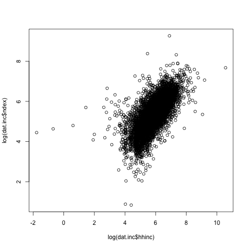
Base R plots

plot(y = log(dat.inc$ndex), x = log(dat.inc$hhinc))  # many options. see ?plot and ?par

## Warning: NaNs produced

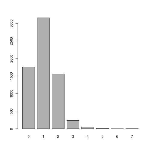
plot(factor(dat.inc$ncars))  # plot depends on data types

Plots with ggplot

• ggplots are based on the Grammar of Graphics
• click here for help, examples and tutorials at http://ggplot2.org/
• a plot is defined by a set of data that is mapped onto a picture - in many complicated ways, if you so desire
• the mappings are called aes() thetics. For example aes(x=var1,y=var2)
• the way they appear in the picture are called geom etrics
• there is a very long list of geoms. Refer to documentation.
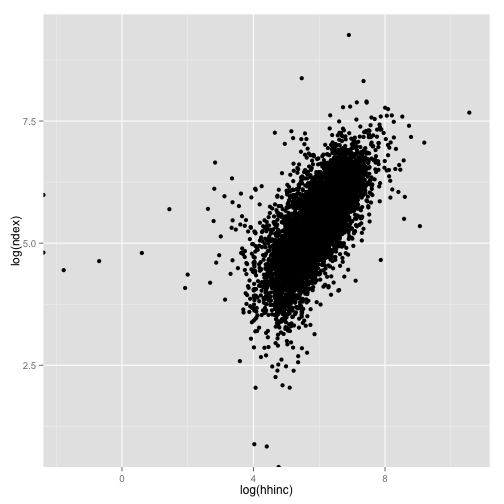
• let’s plot log non-durable expenditure against log household income in a scatter plot

library(ggplot2)
p <- ggplot(data = dat.inc, aes(x = log(hhinc), y = log(ndex)))  # not a plot yet: misses a geom
p + geom_point()  # now that's a plot

## Warning: NaNs produced

## Warning: NaNs produced

## Warning: Removed 4 rows containing missing values (geom_point).

ggplot 2

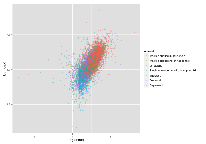
dat <- subset(dat.inc, hhinc > 0 & ndex > 0)  # get rid of some negative values
# add another layer: color points by marstat, and decrease opacity to 0.4
p <- ggplot(data = dat, aes(x = log(hhinc), y = log(ndex)))  # not a plot yet: misses a geom
p + geom_point(aes(color = marstat), alpha = 0.4)

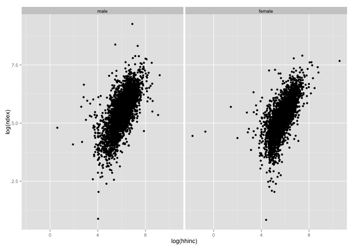
p + geom_point() + facet_wrap(~sex)  # split plot by factor sex

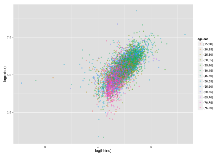
More ggplots

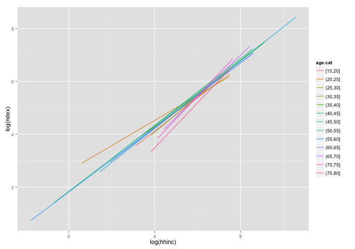
ggplot(data = dat, aes(x = log(hhinc), y = log(ndex))) + geom_point(aes(color = age.cat), 
    alpha = 0.4)

ggplot(data = dat, aes(x = log(hhinc), y = log(ndex))) + geom_smooth(aes(color = age.cat), 
    method = "lm", se = FALSE)

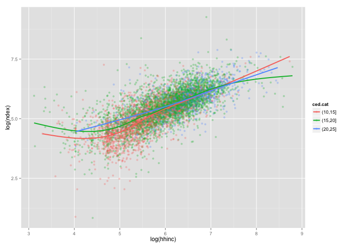
sdat <- subset(dat, ced.cat %in% c("(10,15]", "(15,20]", "(20,25]") & 
    log(hhinc) > 3 & log(hhinc) < 9)  # select a subset of ced
ggplot(data = sdat, aes(x = log(hhinc), y = log(ndex))) + geom_point(aes(color = ced.cat), 
    alpha = 0.3) + geom_smooth(aes(color = ced.cat), se = FALSE, size = 1)

## geom_smooth: method="auto" and size of largest group is >=1000, so using
## gam with formula: y ~ s(x, bs = "cs"). Use 'method = x' to change the
## smoothing method.

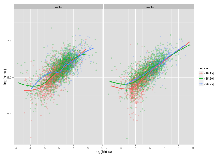
# split by sex?
ggplot(data = sdat, aes(x = log(hhinc), y = log(ndex))) + geom_point(aes(color = ced.cat), 
    alpha = 0.3) + geom_smooth(aes(color = ced.cat), se = FALSE, size = 1) + 
    facet_wrap(~sex)

## geom_smooth: method="auto" and size of largest group is >=1000, so using
## gam with formula: y ~ s(x, bs = "cs"). Use 'method = x' to change the
## smoothing method.

## geom_smooth: method="auto" and size of largest group is >=1000, so using
## gam with formula: y ~ s(x, bs = "cs"). Use 'method = x' to change the
## smoothing method.

Regression Models

• linear models: lm()
• generalized linear models (probit, logit et al): glm
• loads of packages on CRAN
• specify a model with a formula

mod.1 <- lm(formula = lndex ~ log(hhinc), data = dat)
summary(mod.1)

## 
## Call:
## lm(formula = lndex ~ log(hhinc), data = dat)
## 
## Residuals:
##    Min     1Q Median     3Q    Max 
## -3.481 -0.307 -0.004  0.309  4.467 
## 
## Coefficients:
##             Estimate Std. Error t value Pr(>|t|)    
## (Intercept)  1.22476    0.05123    23.9   <2e-16 ***
## log(hhinc)   0.70251    0.00859    81.8   <2e-16 ***
## ---
## Signif. codes:  0 '***' 0.001 '**' 0.01 '*' 0.05 '.' 0.1 ' ' 1 
## 
## Residual standard error: 0.556 on 6776 degrees of freedom
## Multiple R-squared: 0.497,   Adjusted R-squared: 0.497 
## F-statistic: 6.7e+03 on 1 and 6776 DF,  p-value: <2e-16

update() a model

• easy to iterate on models

mod.2 <- update(mod.1, . ~ . - 1)  # leave formula as is, but substract the intercept
mod.3 <- update(mod.1, . ~ . + age + I(age^2))  # add age and age squared
coef(summary(mod.2))  # use coef() function to extract coefs only

##            Estimate Std. Error t value Pr(>|t|)
## log(hhinc)    0.906   0.001179   768.5        0

coef(summary(mod.3))

##               Estimate Std. Error t value  Pr(>|t|)
## (Intercept)  0.9492539  7.710e-02   12.31 1.805e-34
## log(hhinc)   0.6422908  8.854e-03   72.55 0.000e+00
## age          0.0336750  2.667e-03   12.62 3.942e-36
## I(age^2)    -0.0003756  2.525e-05  -14.88 2.767e-49

predict() data from a model

• use the predict() function
• most regression functions have got their own prediction method.
• say we want to predict values of lndex from mod.3

newdat <- expand.grid(hhinc = c(200, 300), age = c(20, 50, 80))
cbind(newdat, predict(mod.3, newdat))

##   hhinc age predict(mod.3, newdat)
## 1   200  20                  4.876
## 2   300  20                  5.136
## 3   200  50                  5.097
## 4   300  50                  5.358
## 5   200  80                  4.643
## 6   300  80                  4.903

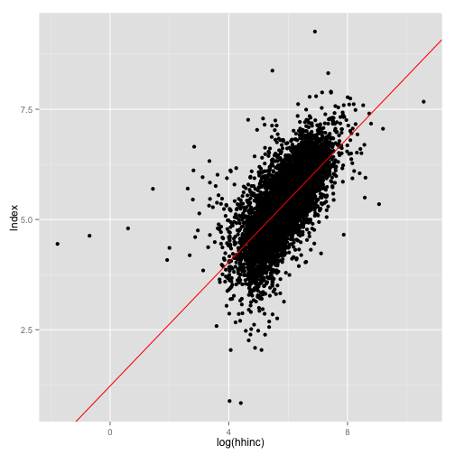
ggplot model coeficients

• abline() is a convenient geom for this
• works well for single explanatory variable

p <- ggplot(dat, aes(x = log(hhinc), y = lndex))
p + geom_point() + geom_abline(intercept = coef(mod.1)[1], slope = coef(mod.1)[2], 
    col = "red")

update() a model 2: add a dummy variable

• let’s add the number of rooms as a dummy variable d
• i.e. we want d1=1 if nrooms==1, d1=0 else; d2=1 iff nrooms==2 etc
• R does that for you (you don’t want to create all those d’s)

mod.4 <- update(mod.3, . ~ . + factor(nrooms))
summary(mod.4)

## 
## Call:
## lm(formula = lndex ~ log(hhinc) + age + I(age^2) + factor(nrooms), 
##     data = dat)
## 
## Residuals:
##    Min     1Q Median     3Q    Max 
## -3.751 -0.307 -0.008  0.303  3.477 
## 
## Coefficients:
##                  Estimate Std. Error t value Pr(>|t|)    
## (Intercept)      9.09e-01   1.64e-01    5.56  2.9e-08 ***
## log(hhinc)       5.74e-01   9.36e-03   61.37  < 2e-16 ***
## age              2.66e-02   2.64e-03   10.09  < 2e-16 ***
## I(age^2)        -3.16e-04   2.49e-05  -12.72  < 2e-16 ***
## factor(nrooms)2  3.37e-01   1.58e-01    2.13  0.03334 *  
## factor(nrooms)3  3.12e-01   1.48e-01    2.11  0.03504 *  
## factor(nrooms)4  5.27e-01   1.47e-01    3.59  0.00034 ***
## factor(nrooms)5  5.91e-01   1.47e-01    4.02  5.9e-05 ***
## factor(nrooms)6  7.53e-01   1.47e-01    5.12  3.1e-07 ***
## ---
## Signif. codes:  0 '***' 0.001 '**' 0.01 '*' 0.05 '.' 0.1 ' ' 1 
## 
## Residual standard error: 0.526 on 6769 degrees of freedom
## Multiple R-squared: 0.55,    Adjusted R-squared: 0.549 
## F-statistic: 1.03e+03 on 8 and 6769 DF,  p-value: <2e-16

Hyothesis Testing, IV models

• check out library(car) and library(AER)
• convenient functions for all applied econometrics tasks

Create an Age Profile for consumption

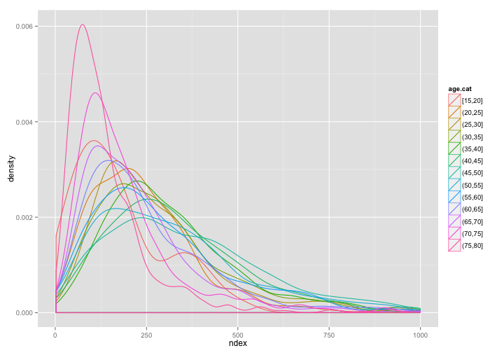
• How does the distribution of non-durable expenditure vary wity age?
• How to model this in a regression model?

ggplot(subset(dat, ndex < 1000), aes(x = ndex)) + geom_density(aes(color = age.cat))

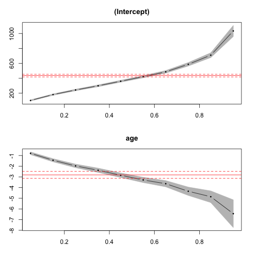
Age Profile: Quantile Regression

library(quantreg)
qreg50 <- rq(formula = ndex ~ age, data = dat, tau = 0.5)  # median regression
qreg <- rq(formula = ndex ~ age, data = dat, tau = seq(0.05, 0.95, 
    le = 10))  # quantile reg at several quantiles
plot(summary(qreg))  # very nice plotting method

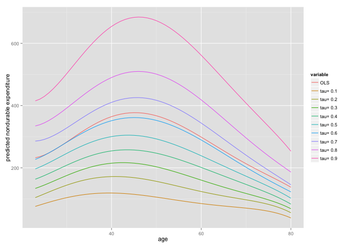
Age Profile: Compare OLS and Quantile Reg

• compare the Conditional Expectation (the OLS estimate) with the conditional quantile function
• fit a 5-th order polynomial in age

form    <- ndex ~ age + I(age^2) + I(age^3) + I(age^4) + I(age^5)
lin.mod <- lm(formula = form, data=dat)
taus    <- seq(0.1,0.9,le=9) # desired quantiles
qr.mod  <- rq(formula= form,data=dat,tau=taus)
ages    <- sort(unique(dat$age)) # vector of ages in data
# create data.frame with cols "age", and a prediction for each model
preds   <- data.frame(age = ages, OLS= predict(lin.mod, newdata = data.frame(age = ages)))
# add qreg predictions
preds   <- cbind(preds, predict(qr.mod,data.frame(age=ages)))
head(preds)

##   age   OLS tau= 0.1 tau= 0.2 tau= 0.3 tau= 0.4 tau= 0.5 tau= 0.6 tau= 0.7
## 1  17 267.1    51.39    78.01    122.5    150.5    186.3    221.6    336.6
## 2  18 252.6    54.85    80.65    121.0    149.3    183.9    217.6    318.8
## 3  19 242.2    58.70    84.21    121.2    149.7    183.4    215.9    305.4
## 4  20 235.4    62.85    88.51    122.8    151.5    184.7    216.2    295.8
## 5  21 231.7    67.20    93.42    125.5    154.5    187.4    218.4    289.6
## 6  22 230.9    71.66    98.77    129.3    158.6    191.5    222.1    286.5
##   tau= 0.8 tau= 0.9
## 1    371.4    484.3
## 2    355.9    457.0
## 3    344.8    437.0
## 4    337.5    423.5
## 5    333.6    415.9
## 6    332.8    413.3

Plot OLS vs Quantile Reg Age Profiles

• ggplot works best with long data.
• need to reshape preds into long

library(reshape)
mpreds <- melt(preds, id.vars = "age")  # now the data is long
head(mpreds)

##   age variable value
## 1  17      OLS 267.1
## 2  18      OLS 252.6
## 3  19      OLS 242.2
## 4  20      OLS 235.4
## 5  21      OLS 231.7
## 6  22      OLS 230.9

ggplot(subset(mpreds, age > 22), aes(x = age, y = value, color = variable)) + 
    geom_line() + scale_y_continuous(name = "predicted nondurable expenditure")

R and Time Series

• R has strong time series capabilities
• base time series architecture in ts()
• more advanced ways to deal with time/date classes
  • Lubridate
  • xts
• check out
  • CRAN Time Series Task View: General Overview
  • library(zoo) for general ordered obs
  • library(dynlm) for dynamic regressions

data(UKDriverDeaths)
UK <- UKDriverDeaths
str(UK)

##  Time-Series [1:192] from 1969 to 1985: 1687 1508 1507 1385 1632 ...

plot(UK)

plot(decompose(UK))

acf(UK)

pacf(UK)

R and panel data

• package plm
• others…

R and multinomial logit

• mlogit package

R and Foreign Languages

• It is easy to call other languages from within R
• R is itself written in Fortran and C, so those two are particularly easy
• This is important for R users who want a lot of performance (MCMC, dynamic programming, etc)

R and Fortran

• suppose we have the fortran submodule bar.f stored on disk
• it takes integer n, makes x=1:n and returns x^2
• it looks like that

    subroutine bar(n, x)
        integer n
        double precision x(n)
        integer i
        do 100 i = 1, n
            x(i) = x(i) ** 2 
    100 continue
    end

• we need to compile the function. write in your terminal

cd ~/git/R-demo
R CMD SHLIB bar.f

• It’s already compiled in the github repository so no need to if you downloaded that.
• finally, in R we need to load the dynamic library and call the function

dyn.load("bar.so")
how.many <- 5L # L means integer
y        <- rnorm(how.many)
r.result <- y^2
# ideally we have a wrapper on .Fortran to check sanity of input
f.result <- .Fortran("bar", n=how.many, x=y) # .Fortran returns a list
identical(r.result,f.result$x) #identical?

## [1] TRUE

R and C/C++

• library(Rcpp)
• Rcpp Mastermind Dirk Eddelbuettel
• you can write packages the use C code via Rcpp
• very useful if you have a part of your code that needs speeding up.
• many derived libraries
  • library(RcppArmadillo): interface to the Armadillo C++ matrix algebra library. Armadillo is close to matlab.
  • library(RcppEigen): interface to the C++ Eigen libraries. Eigen is a very versatile matrix algebra library. Great for sparse matrices.
  • library(RcppSimpleTensor): High dimensional computations made easy
  • many more
• you can write C code inline and test it

R and C++ inline

• library(inline) allows inline testing of C code

library(inline)
my.cpp.code <- "NumericVector xx(x); 
                return wrap( std::accumulate( xx.begin(), xx.end(), 0.0));"
my.cpp.fun  <- cxxfunction( signature( x="numeric"), body=my.cpp.code, plugin="Rcpp")
y           <- seq(1,10,0.5)
r.result    <- sum(y)
c.result    <- my.cpp.fun(y)
identical(r.result,c.result)

## [1] TRUE

# if you want to see what's going on under the hood:
my.cpp.fun  <- cxxfunction( signature( x="numeric"), body=my.cpp.code, plugin="Rcpp", verbose=TRUE)

##  >> setting environment variables: 
## PKG_LIBS =  /Library/Frameworks/R.framework/Versions/2.15/Resources/library/Rcpp/lib/x86_64/libRcpp.a
## 
##  >> LinkingTo : Rcpp
## CLINK_CPPFLAGS =  -I"/Library/Frameworks/R.framework/Versions/2.15/Resources/library/Rcpp/include" 
## 
##  >> Program source :
## 
##    1 : 
##    2 : // includes from the plugin
##    3 : 
##    4 : #include <Rcpp.h>
##    5 : 
##    6 : 
##    7 : #ifndef BEGIN_RCPP
##    8 : #define BEGIN_RCPP
##    9 : #endif
##   10 : 
##   11 : #ifndef END_RCPP
##   12 : #define END_RCPP
##   13 : #endif
##   14 : 
##   15 : using namespace Rcpp;
##   16 : 
##   17 : 
##   18 : // user includes
##   19 : 
##   20 : 
##   21 : // declarations
##   22 : extern "C" {
##   23 : SEXP file90625393cbd( SEXP x) ;
##   24 : }
##   25 : 
##   26 : // definition
##   27 : 
##   28 : SEXP file90625393cbd( SEXP x ){
##   29 : BEGIN_RCPP
##   30 : NumericVector xx(x); 
##   31 :                 return wrap( std::accumulate( xx.begin(), xx.end(), 0.0));
##   32 : END_RCPP
##   33 : }
##   34 : 
##   35 : 
## Compilation argument:
##  /Library/Frameworks/R.framework/Resources/bin/R CMD SHLIB file90625393cbd.cpp 2> file90625393cbd.cpp.err.txt

How to report results

• knitr
• reproducible research

How to make this set of slides

• Use RStudio to author an R markdown file
• click a button in RStudio to knit an HTML document
• this uses the amazing knitr package to “knit” (evaluated or not) R code into text documents.
• finally use pandoc to convert to HTML5 slides: pandoc -s -S -t slidy --mathjax intro.md -o intro.html
• Get the R markdown source code of this presentation on github
• More info at MAGES blog