Risk processes with tax
Dalal Al Ghanim
Ronnie Loeffen
Alex Watson
· UCL Stats Internal Seminar, 17 July 2020
- Loss-carry-forward: tax paid at the maximum
- What is the best tax rate to maximise revenue?
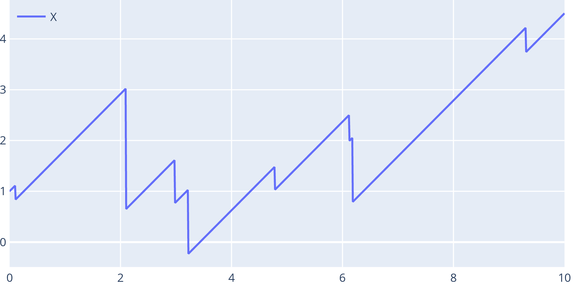
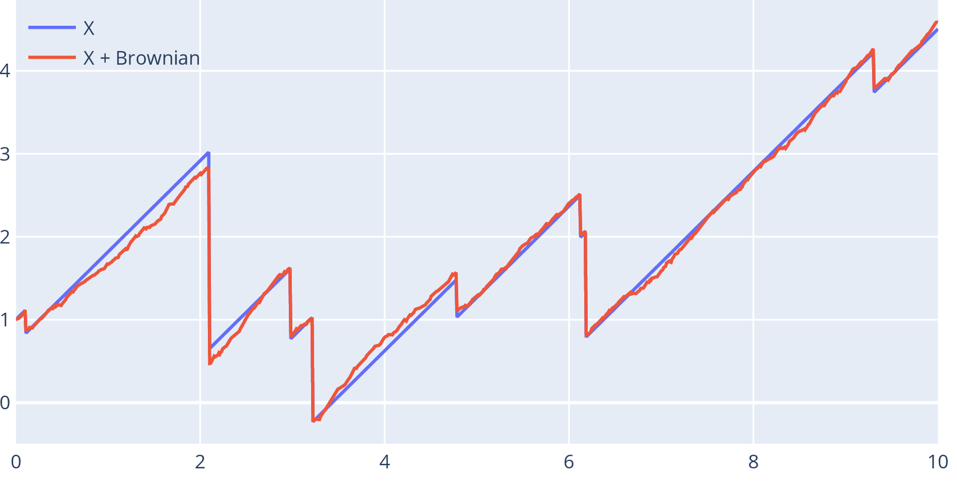
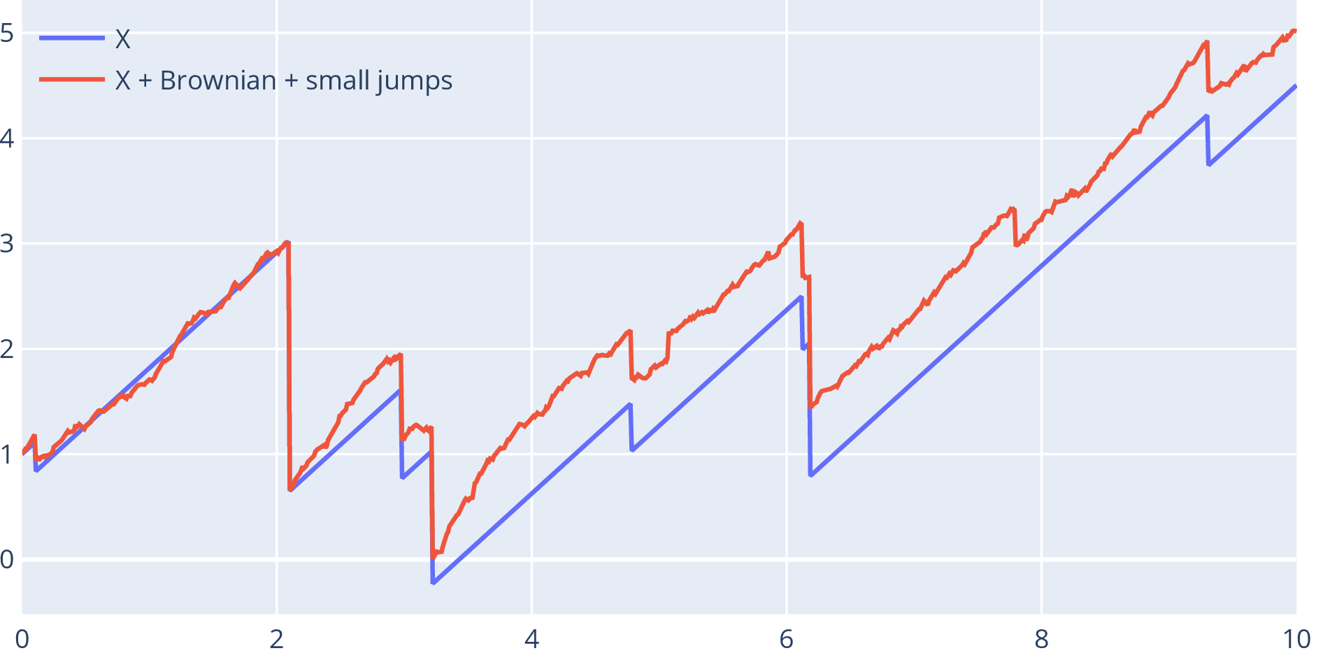
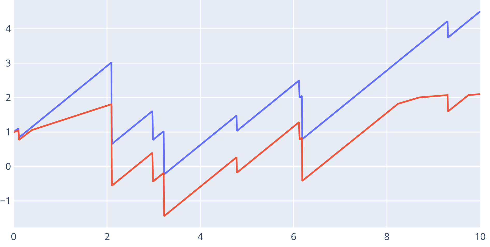
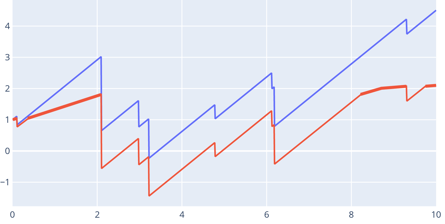
- Risk process: with Poisson process, i.i.d.
- Can include Brownian part and fast, small jumps : Lévy process
- Wealth of insurance company: is premium rate, are claims
- Intrinsic motivation: continuous equivalent of random walk
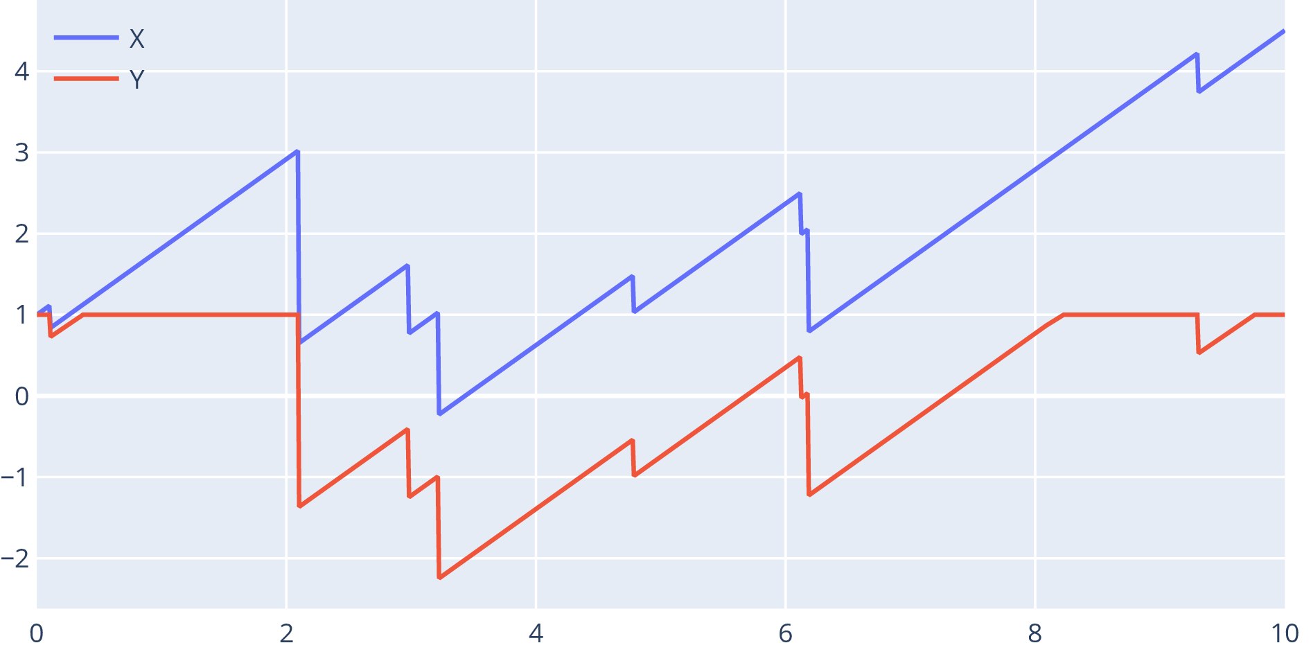
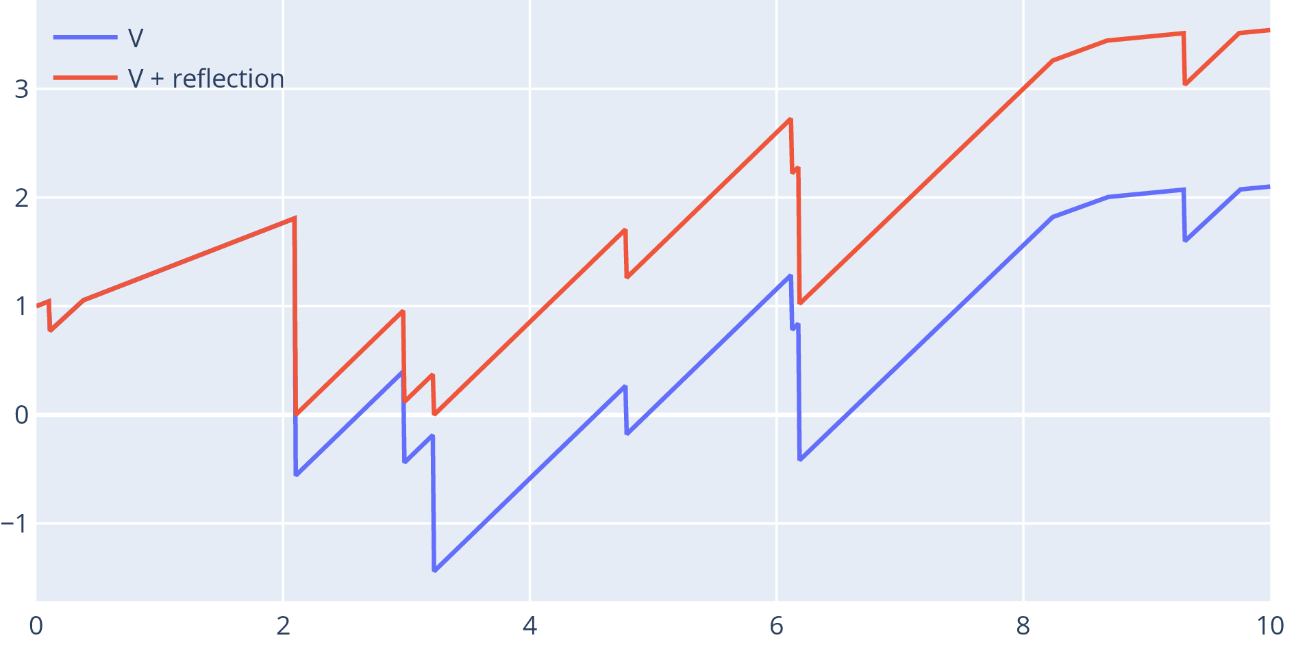
Tax process – partially reflected

- is the tax rate in loss-carry-forward taxation
- Introduces spatial dependence in a tractable way
- Questions: existence? computation of functionals? optimal ?
Two ideas in literature:
- – not obvious it exists – is Markov
- – clear that it exists – is not Markov
Theorem – Al Ghanim, Loeffen, W. (2020)
If the differential equation
has a unique solution, then the equation
has a unique solution .
- Let .
- satisfies the equation for : existence
- Converse direction: uniqueness
- Core idea: look at and while they are drifting at the maximum
Theorem – Al Ghanim, Loeffen, W. (2020+)
Assume , for , satisfies:
- if or ,
- if ,
where is the generator of (acting on coordinate ). Then, .
for is the condition for to be in the domain of the generator of
- Apply to get
where are scale functions (with known Laplace transform).
- Not the only way, but:
- Flexible
- Can guess with some dodgy method, and verify with the theorem
- Reduces need for excursion theory or approximation by bounded variation processes
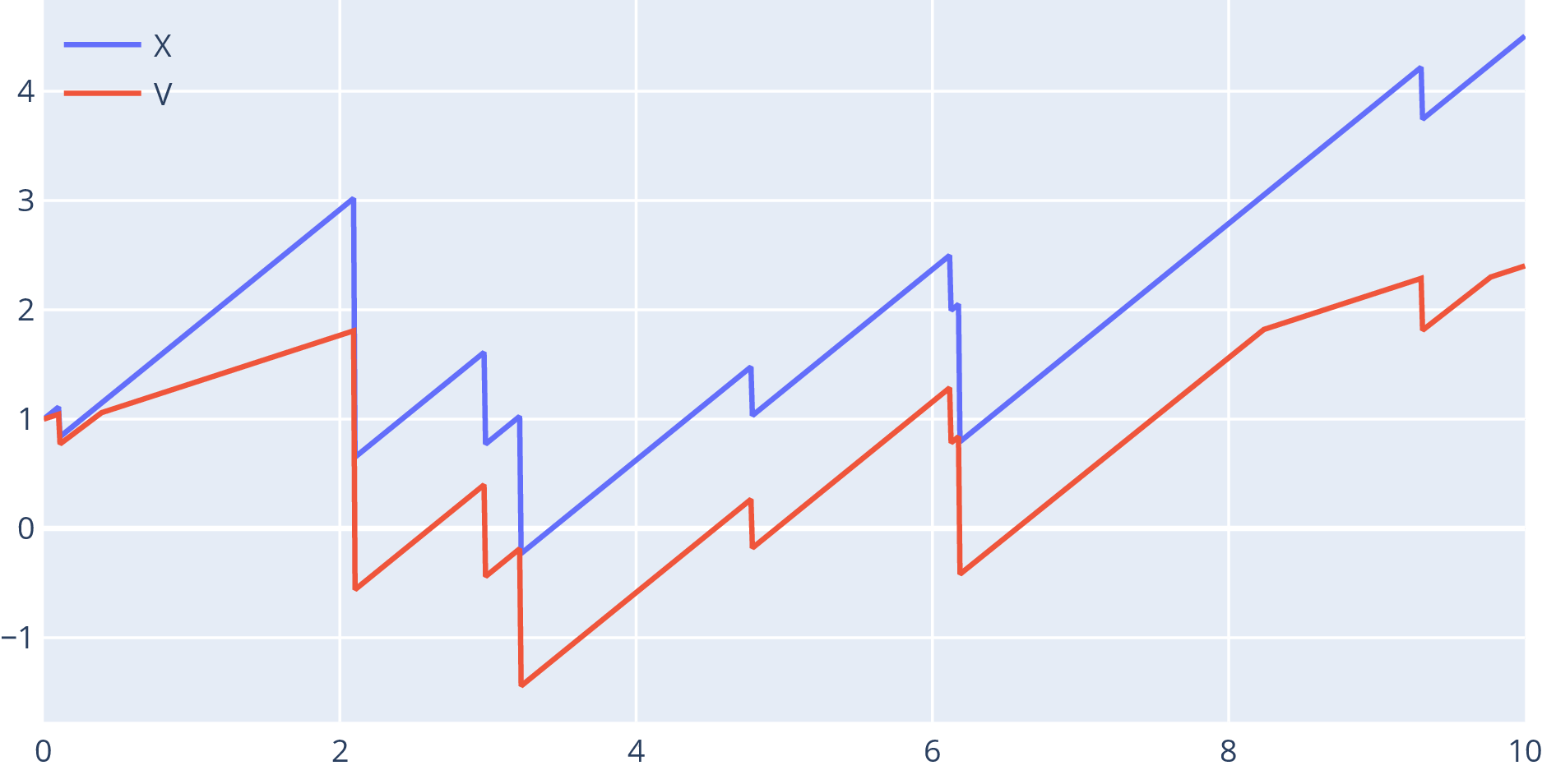
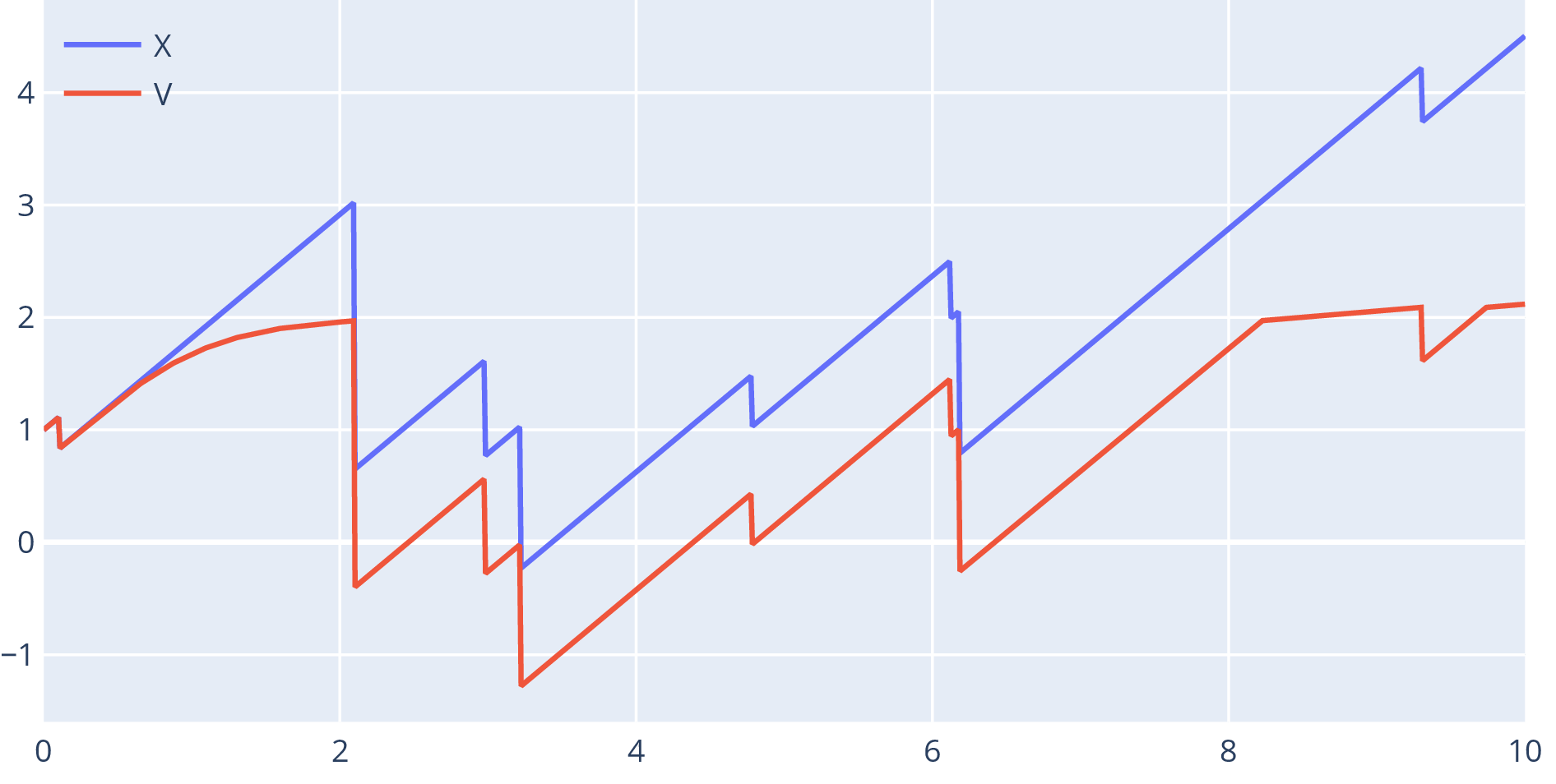
- Process reflected below at zero: ‘capital injections’ or ‘bail-outs’
- Conditions for ‘’
are:
- if , and if ,
- if ,
- Only change is in boundary conditions
- What is the best tax rate to maximise revenue?
- For a predictable process, define , under which
- If , this is a tax process
- If totally free to choose: reflection above (at some level), i.e.
- If tax rate constrained to :
switch from
to when
crosses
some level ,
i.e. ,
- Extension to maximising tax revenue minus bail-out cost, etc. – many possibilities
- Solutions are explicit (in terms of scale functions)
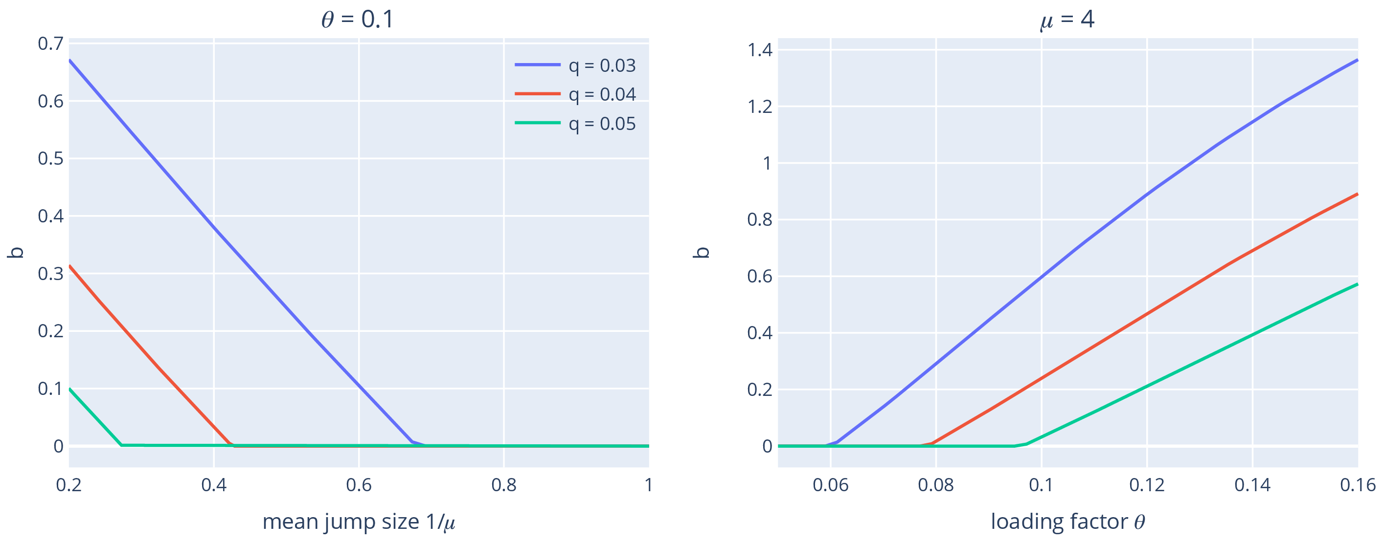
Optimal control: explicit result
- Assumption: the tail of the Lévy measure is log-convex
- Think of the Lévy measure as , where is the rate of the Poisson process of jumps, and is the distribution of the jumps
- Optimal taxation is of form
- Let
- iff , otherwise is the unique root of
A quirk, or, didn’t someone do this 8 years ago?
- Wang and Hu (IME, 2012): optimal control of tax rates
- Their solution is equivalent to ours
- But it is expressed in terms of an optimal
- Years later we showed and tax rates are equivalent (1st theorem from today)
- We optimise over all tax rates (predictable )
- a -Poisson process; i.i.d. exponential with rate (mean )
- is ‘loading factor’: ,
References
[1] D. Al Ghanim, R. Loeffen and A. R. Watson The equivalence of two tax processes Insurance Math. Econom., 2020. doi:10.1016/j.insmatheco.2019.10.002.
Thank you!