7.01 Covering spaces
Video
Below the video you will find accompanying notes and some pre-class questions.
- Next video: 7.02 Path-lifting, monodromy.
- Index of all lectures.
Notes
Intuition for covering spaces
(0.30) Take \(\mathbf{C}\setminus\{0\}\) and consider the map \(p\colon\mathbf{C}\setminus\{0\}\to\mathbf{C}\setminus\{0\}\) given by \(p(z)=z^2\). This map is surjective and 2-to-1. Nonetheless, we do have something like an inverse locally: the square root function (we actually have two local inverses differing by a sign \(\pm\sqrt{}\)).
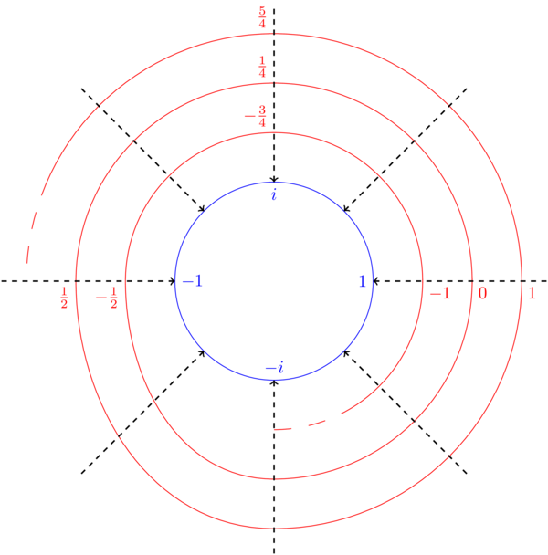
(2.26) More precisely, if we excise a half-line \(B=\{z\in\mathbf{C}\setminus\{0\}\ :\ Im(z)=0,\ Re(z)<0\}\) then on \(\mathbf{C}\setminus B\) we have two functions \[q_+,q_-\colon\mathbf{C}\setminus B\to\mathbf{C}\setminus\{0\}\] such that \(p(q_\pm(z))=z\). In this example, \(q_-=-q_+\), e.g.\(q_+(1)=1\), \(q_-(1)=-1\).
(4.00) We could equally have taken a branch cut \(\{z\in\mathbf{C}\setminus\{0\}\ :\ Im(z)=0,\ Re(z)>0\}\) and we would have obtained two different local inverses for \(p\). The point of taking a branch cut is that \(\mathbf{C}\setminus\{0\}\) is not simply-connected but \(\mathbf{C}\setminus B\) is simply-connected, which is what lets us define an inverse on the complement of the branch-cut.
(5.11) Take \(f\colon\mathbf{C}\mapsto\mathbf{C}\setminus\{0\}\), \(f(z)=e^{iz}\). This map is surjective and \(\infty\)-to-1 (for example \(f^{-1}(1)=\{2\pi n\ :\ n\in\mathbf{Z}\}\)). On the complement of a branch cut \(B\) we have infinitely many well-defined local inverses \(q_n=2\pi n-i\log)\colon\mathbf{C}\setminus B\to\mathbf{C}\) satisfying \(q_n(1)=2\pi n\) and \(p(q_n(z))=z\) (that is \(\exp(i(2\pi n-i\log z))=z\)). [The video is missing a factor of \(-i\).]
(9.00) Roughly speaking, a covering map is a map \(p\colon Y\to X\) which is \(N\)-to-1 for some \(N\) and which has \(N\) locally-defined inverses \(q_n\) defined on simply-connected subsets of the target (satisfying \(p\circ q_n=id\)).
(10.40) Notice that in the second example, the domain of the covering map is \(\mathbf{C}\), which is simply-connnected, and the local inverses \(q_n\) are indexed by the integers \(\mathbf{Z}\). This is, roughly speaking, how you deduce that the target of the covering map has \(\pi_1\cong\mathbf{Z}\).
Definition
(11.20) Let \(p\colon Y\to X\) be a continuous map.
- A subset \(U\subset X\) is called an elementary neighbourhood if
there is a discrete set \(F\) and a homeomorphism \(h\colon
p^{-1}(U)\to U\times F\) such that \(pr_1\circ h=p|_{p^{-1}(U)}\)
(where \(pr_1\colon U\times F\to U\) is the projection to the
first factor).
- (13.30) You should think of an elementary neighbourhood as playing the role of the complement of a branch cut in our earlier examples: \(U\) is the subset on which you have locally-defined inverses to \(p\).
- (13.57) The locally-defined inverses are parametrised by the discrete set \(F\); in our examples we had \(F=\{-1,1\}\) and \(F=\mathbf{Z}\). For each point \(m\in F\) we get a map \(q_m\colon U\to U\times F\to p^{-1}(U)\) defined by \(q_m(x)=h^{-1}(x,m)\) which satisfies \(p(q_m(x))=pr_1(h(h^{-1}(x,m)))=x\).
- (16.07) We say \(p\) is a covering map if \(X\) is covered by
elementary neighbourhoods (i.e. every point \(x\in X\) is
contained in some elementary neighbourhood).
- Note that the word cover can now mean two things: covering map and open cover (like in the definition of compactness). Hopefully it will be clear what is meant from the context.
- (17.40) We say that a subset \(V\subset Y\) is an elementary sheet if it is path-connected and \(p(V)\) is an elementary neighbourhood.
(18.36) Here is a picture of the exponential map \(p(z)=e^{iz}\) restricted to the real axis (so its image is the unit circle in \(\mathbf{C}\)):
We draw the domain as a helix living over the circle (winding around infinitely often). In the circle, the green arc is an elementary neighbourhood (complement of a branch cut). Its preimage is a union of infinitely many arcs, each of which is an elementary sheet.
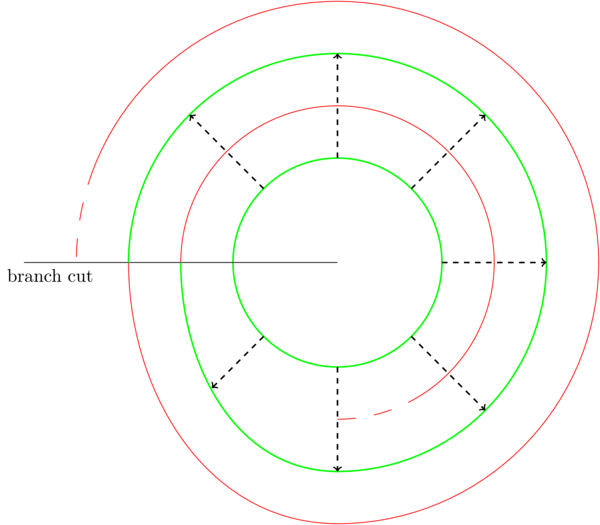
(21.30) Here is a picture of the squaring map \(p_2(z)=z^2\) (restricted to the unit circle). In the circle, the green arc is an elementary sheet; its preimage is a union of two arcs, each of which is an elementary sheet.

More generally, the map \(p_n(z)=z^n\) would give a helix with \(n\) turns (\(n=3\) in the picture):

More examples
(24.05) Consider the figure 8, with its two loops drawn in red and blue. The following picture defines a 2-to-1 covering space of the figure 8:
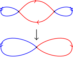
We see that the cross-point of the figure 8 has two preimages each of which looks like the cross point. The preimage of the blue edge consists of two blue edges upstairs in the covering space. The preimage of the red edge consists of two red edges upstairs. Each edge maps down to the corresponding edge in the figure 8 in such a way that the arrows match up. (The arrows do not indicate any identifications being made).
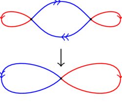
(26.22) Another covering space of the figure 8 is given by this picture:
Pre-class questions
- Are there any other 2-to-1 covers of the figure 8? Remember, in each case, the cross-point has two preimages which look like cross-points, each edge has two preimages which connect the cross-points.
Navigation
- Next video: 7.02 Path-lifting, monodromy.
- Index of all lectures.