Elliptic function slide rule

To me, elliptic functions have always sounded exotic and mysterious. They're related to modular forms. They appear in period calculations for Hamiltonian systems. They allow you to solve some complicated integrable systems like geodesics on an ellipsoid. They always seemed like a relic from a bygone age of heroic calculation. In fact, the definition of the Jacobi elliptic functions is very geometric, essentially a small modification of the SOHCAHTOA definition of the trigonometric functions.

Consider an ellipse of eccentricity \(k\), that is, the curve \(x^2+y^2/b^2=1\) with \(k^2=1-1/b^2\). You can try and parametrise this by arc-length.

If \(k=0\) (so you have the unit circle) then we know the arc-length parametrisation is \((x(s),y(s))=(\cos(s),\sin(s))\) (because the angle measured in radians is precisely the arc-length of a unit circle segment subtending this angle).

For an ellipse with \(k\neq 0\), we get \((r(s)\cos\theta(s),r(s)\sin\theta(s))\) where \(r(s)\) and \(\theta(s)\) are functions of the arc-length: \(r(s)\) is called \(nd(s,k^2)\) and \(\theta(s)\) is called \(am(s,k^2)\) (the "Jacobi amplitude function"). Note that in writing \(r,\theta\), we were suppressing the dependence on the eccentricity (because we were imagining the ellipse to be fixed). We also get the functions \(cn(s,k^2)=\cos\theta(s)\) and \(sn(s,k^2)=\sin\theta(s)\).

There are also functions \(dn=1/nd\), \(nc=1/cn\) and \(ns=1/sn\) and various other combinations, all of which have some geometric interpretation (just like the secant or cosecant have for a circle). All of these are examples of elliptic functions.

So how might you depict these functions usefully on a slide rule? We will use \(am(s,k^2)\) as an angular coordinate and \(\epsilon+k^2\) as a radial coordinate. Since \(k^2\in[0,1)\), our picture will fit onto the annulus between radii \(\epsilon\) and \(\epsilon+1\). Draw the lines of constant \(s\), that is the parametric curves \(\{(1+k^2)cn(s,k^2),(1+k^2)sn(s,k^2))\ :\ k\in[0,1)\}\) on this annulus. If you want to compute \(am(s,k^2)\), for example, all you need to do is to take the circle of radius \(k^2\), intersect it with the correct contour of constant \(s\) and measure the angle this point makes with the horizontal. I think of this as a (circular) slide rule because you make your measurements by superimposing a circular protractor on the annulus described above.

What I realised this morning is that as \(s\) increases, the contours of constant \(s\) behave rather strangely. When \(k=0\), we know that \(am(s,0)=s\) (because the arc-length agrees with the angle in radians for a circle). This means our contours start off looking like radii near the inner boundary of the annulus. However, if we fix an amount of arc-length, this is traced out very quickly (in a very small angle) by an ellipse with sufficiently large eccentricity. In other words, all of our contours bend back around towards the positive \(x\)-axis. By the time you get to arc-length \(2\pi\), your contour starts to look like the result of Dehn twisting the positive \(x\)-axis around the core circle of your annulus.

Here is a plot which hopefully demonstrates what I mean…

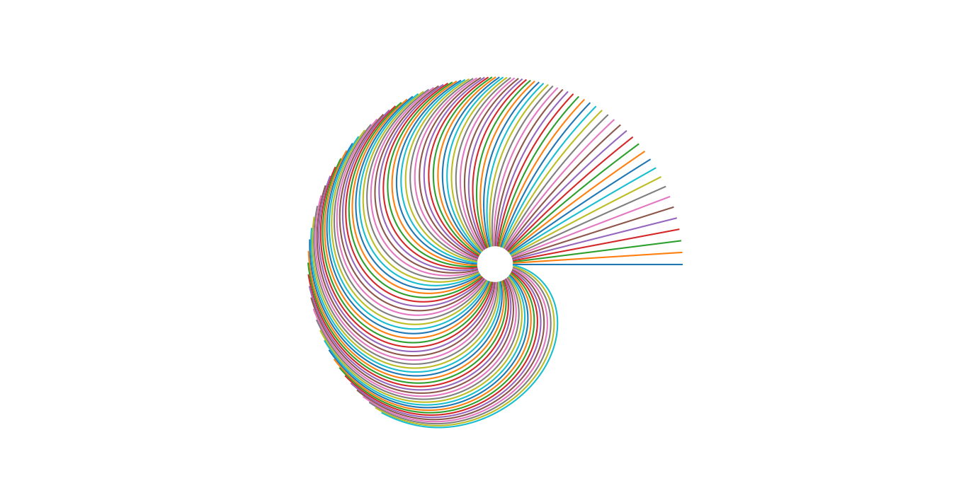
…and here is the Python code used to generate the plot.

#!/usr/bin/python3
import matplotlib.pyplot as plt
import numpy as np
import scipy.special as sf

def sn(u,m):
    return sf.ellipj(u,m)[0]

def cn(u,m):
    return sf.ellipj(u,m)[1]


fig = plt.figure()
ax = fig.add_subplot(111)

for k in range(0,100):
    u=2*np.pi*k/100
    m=np.linspace(0,0.9,1000)
    plt.plot((0.1+m)*cn(u,m),(0.1+m)*sn(u,m))

ax.set_aspect(1)
plt.axis('off')
plt.show()